Part 5: Association Rule Learning
What is Association Rule Learning (ARL) in ML?

(Source: Harshajit Sarmah, 2019)
Association rule learning (ARL) is a rule-based ML method for discovering interesting relationships between variables in large databases and is intended to identify strong rules discovered in databases using some measures of interestingness. It checks for a dependency of one data item on another data item and maps accordingly.
| Transaction ID | milk | bread | butter | beer | diapers |
|---|---|---|---|---|---|
| 1 | 1 | 1 | 0 | 0 | 0 |
| 2 | 0 | 0 | 1 | 0 | 0 |
| 3 | 0 | 0 | 0 | 1 | 1 |
| 4 | 1 | 1 | 1 | 0 | 0 |
| 5 | 0 | 1 | 0 | 0 | 0 |
By definition,
-
Let
represent the set of binary attributes known as items.
- From the example table above, it is the columns where
.
- From the example table above, it is the columns where
-
Let
represent the set of transactions known as database. Each transaction in
has a unique transaction ID and contains a subset of items in
(e.g. transaction with ID
234contains item like milk, butter, bread).- From the example table above, it is the transaction rows where
.
- Note that
, where it is a subset of the database transactions.
- From the example table above, it is the transaction rows where
-
Each rule is defined as an implication of the form
where
.
- Note that
(meaning both sets do not contain any similar items).
- From the example above, a rule can be
(as seen in transaction
4).
- Note that
Support is an indication of how frequently an itemset appears in the database.
To interpret it, we are finding the number of transactions that contains all items of
.
Based on the example data set, the itemset has a support of
1/5 = 0.2 since it occurs in 20% of all transactions.
Confidence is an indication of how often the rule has been found to be true.
To interpret it, we are finding the number of transactions that contains all items of
also contains
.
Based on the example data set, the rule has a confidence of
0.2/0.2 = 1 since it occurs in 100% of all transactions containing butter and bread (one transaction 4).
The lift of a rule is defined as the ratio of the observed support to that expected if and
were independent.
Based on the example data set, the rule has a lift of
0.2/(0.4 * 0.4) = 1.25.
- If the rule has a lift of
= 1, it implies that the probability of occurrence of(antecedent) and
(consequent) are independent of each other, which means no rule can be drawn involving these two events.
- If the rule has a lift of
> 1, it implies the degree to which these two occurrences are dependent on one another, which makes these rules potentially useful for predicting the consequent in future data sets. - If the rule has a lift of
< 1, it implies that the items are a substitute to each other, meaning that the presence of one item has negative effect on the presence of the other (e.g. replacing an item in
Conviction is the ratio of the expected frequency that occurs without
(e.g. the frequency that the rule makes an incorrect prediction).
Based on the example data set, the rule has a conviction of
(1 - 0.4)/(1 - 0.5) = 1.2. This conviction value shows that the rule would be 20% incorrect more often if the association between and
was purely random chance (see transaction
1 not fitting the rule, which is 1/5 = 20% of the total transactions).
-
Apriori Algorithm: Uses frequent data sets to generate association rules, and designed to work on databases that contain transactions. This algorithm uses breadth-first search (BFS) and hash tree to calculate the itemset efficiently.
- Mainly used for market basket analysis to understand products that can be bought together, or healthcare field to find drug reactions for patients.
-
Eclat Algorithm: Stands for Equivalence Class Transformation, it uses a Depth-first search (DFS) to find frequent itemsets in a transaction database.
- Performs faster execution than Apriori algorithm.
-
F-P Growth Algorithm: Stands for Frequent Pattern, it is the improved version of the Apriori algorithm, and represents the database in the form of a tree structure known as a frequent pattern or tree, which purpose is to extract the most frequent patterns.
It is an algorithm that identifies the frequent individual items in the database and extends them to larger item sets as long as these itemsets appear sufficiently often in the database. The frequent itemsets can be used to determine association rules which highlight general trends in the database (e.g. market basket analysis). For the
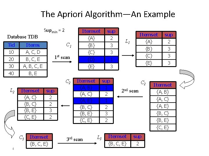
(Source: "Apriori Algorithm Apriori A Candidate Generation Test Approach", n.d.)
A key concept in the Apriori algorithm is the anti-monotonicity of the support measure, and it assumes that (1) all subsets of a frequent itemset must be frequent, (2) and for any infrequent itemset, all its supersets must be infrequent too.
Let's use an example data set,
| Transaction ID | Onion (O) | Potato (P) | Burger (B) | Milk (M) | Beer (Be) |
|---|---|---|---|---|---|
| 1 | 1 | 1 | 1 | 0 | 0 |
| 2 | 0 | 1 | 1 | 1 | 0 |
| 3 | 0 | 0 | 0 | 1 | 1 |
| 4 | 1 | 1 | 0 | 1 | 0 |
| 5 | 1 | 1 | 1 | 0 | 1 |
| 6 | 1 | 1 | 1 | 1 | 0 |
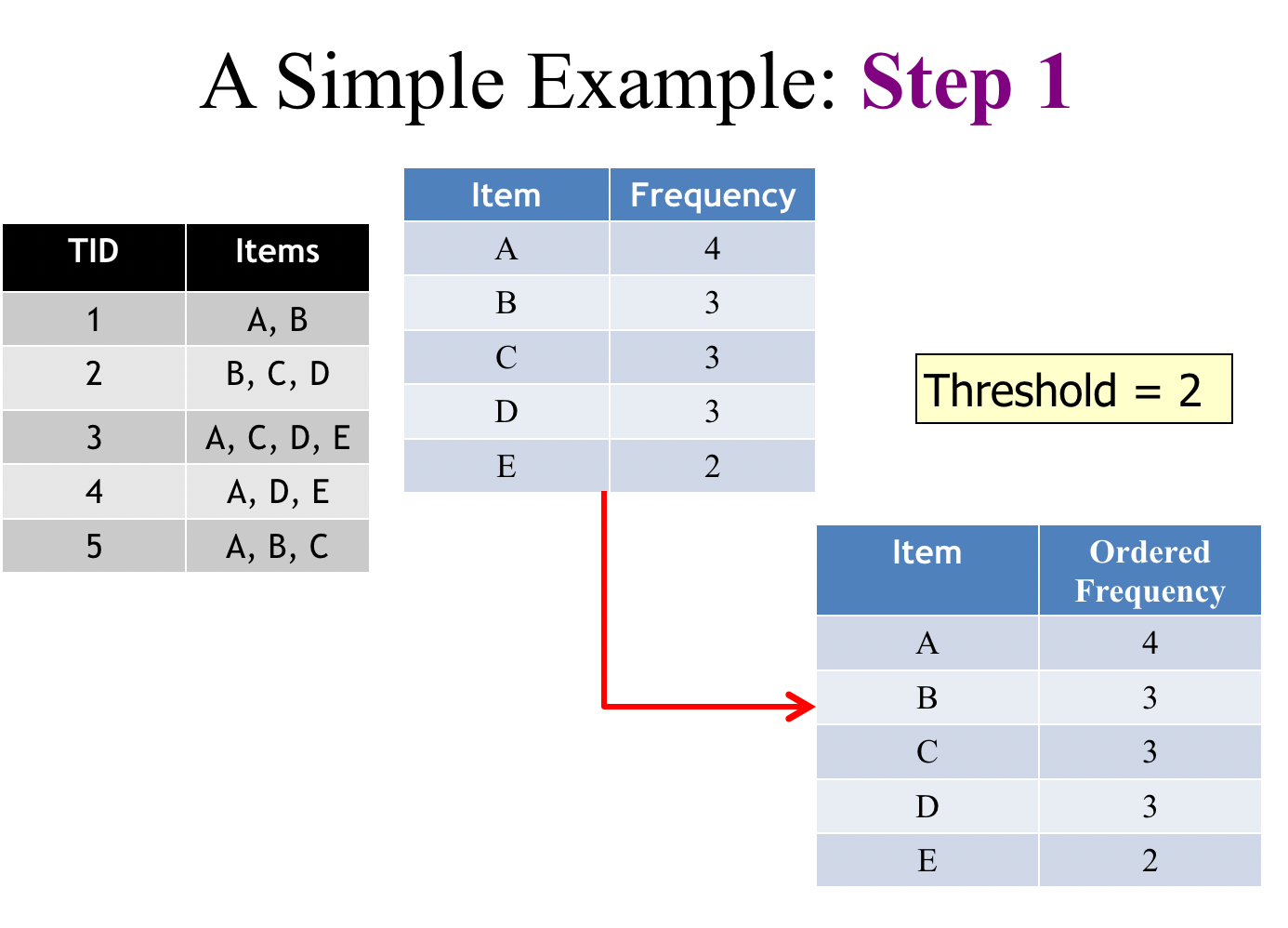
Suppose we set the support threshold to 50% and maximum length (or combination) to 3 and minimum length to 2 (Note that in this example, we are demonstrating using the support threshold, where in reality, confidence and lift thresholds are also considered during the removal process),
For Step 1, create a frequency table of all the items that occur in all the transactions.
| Item | Frequency (No. of transactions) |
|---|---|
| O | 4 |
| P | 5 |
| B | 4 |
| M | 4 |
| Be | 2 |
For Step 2, remove Be since the support level is >=50%, which leaves us to,
| Item | Frequency (No. of transactions) |
|---|---|
| O | 4 |
| P | 5 |
| B | 4 |
| M | 4 |
For Step 3, make a combination of possible pairs without order in mind and duplicates (e.g. {A,B} is the same as {B,A}),
| Itemset | Frequency (No. of transactions) |
|---|---|
| {O,P} | 4 |
| {O,B} | 3 |
| {O,M} | 2 |
| {P,B} | 4 |
| {P,M} | 3 |
| {B,M} | 2 |
For Step 4, remove {O,M} and {B,M} since the support level is >=50%, which leaves us with,
| Itemset | Frequency (No. of transactions) |
|---|---|
| {O,P} | 4 |
| {O,B} | 3 |
| {P,B} | 4 |
| {P,M} | 3 |
For Step 5, use the itemsets found in the prior step to finding a set of three items purchased together by using another rule (called self-join) to pair the itemsets,
- {O,P} and {O,B} gives {O,P,B}
- {P,B} and {P,M} gives {P,B,M}
Then finding the frequency for these two itemsets gives,
| Itemset | Frequency (No. of transactions) |
|---|---|
| {O,P,B} | 3 |
| {P,B,M} | 2 |
Then applying the threshold again, we should derive {O,P,B} as a significant itemset, which means that this set of 3 items was purchased most frequently.
Combined with the set items of length 2, the end result should look like this,
| Itemset | Frequency (No. of transactions) |
|---|---|
| {O,P} | 4 |
| {O,B} | 3 |
| {P,B} | 4 |
| {P,M} | 3 |
| {O,P,B} | 3 |
In summary, the algorithm would be,
- Apply minimum support to find all the frequent sets with
items.
- Use the self-join rule to find the frequent sets with
items with the help of frequent
- Repeat this process from
to the point where the self-join ruel cannot be applied anymore.
(Source: Temple University, 2004)
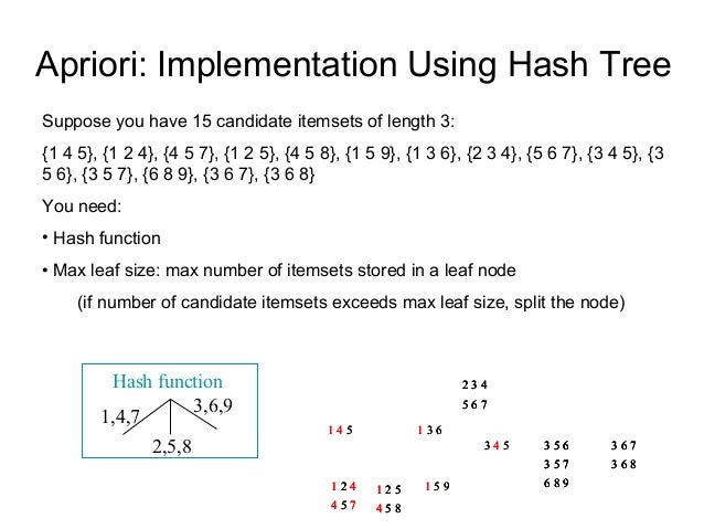
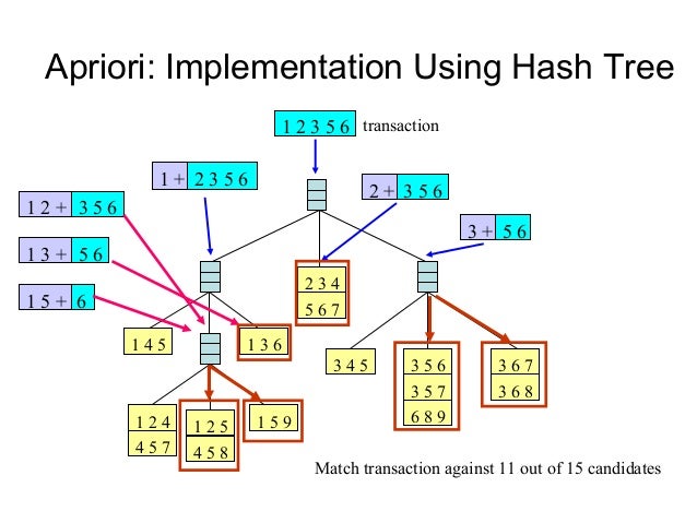
The associated rules are stored in a Hash Tree, and Apriori uses Breadth-First Search (BFS) to mine for the rules. Below is an example of a transversal for BFS,
(Source: Blake Matheny, 2007)
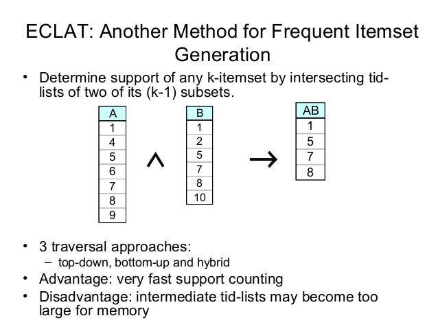
Abbreviated as Equivalence Class clustering and bottom-up LAttice Transversal (ECLAT) algorithm, it finds frequent itemsets in a transaction or database and is known to be one of the best methods of ARL. It uses Depth-First Search (DFS) compared to Apriori which uses Breadth-First Search (BFS), and represents data in a vertical manner, unlike Apriori which represents in a horizontal pattern.
(Source: Temple University, 2004)
Using the same data set from the Apriori description, we restructure the matrix like this for easier reference,
| Item | Transaction IDs |
|---|---|
| O | 1, 4, 5, 6 |
| P | 1, 2, 4, 5, 6 |
| B | 1, 2, 5, 6 |
| M | 2, 3, 4, 6 |
| Be | 3, 5 |
We generate the following combinations, suppose we have a maximum combination of 3 and a minimum combination of 2,
| Itemset | Transaction IDs |
|---|---|
| {O,P} | 1, 4, 5, 6 |
| {O,B} | 1, 5, 6 |
| {P,B} | 1, 2, 5, 6 |
| {P,M} | 2, 4, 6 |
| {B,M} | 2, 6 |
| {M,Be} | 3 |
| {O,M} | 4, 6 |
| {O,Be} | 5 |
| {P,Be} | 5 |
| {B,Be} | 5 |
| {O,P,B} | 1, 5, 6 |
| {P,B,M} | 2, 6 |
| {O,P,M} | 4, 6 |
| {O,P,Be} | 5 |
| {O,B,Be} | 5 |
| {P,B,Be} | 5 |
Then using the same support threshold level of 50% (Note that ECLAT only uses support threshold unlike Apriori which uses several thresholds during the removal process), we get the end result,
| Itemset | Transaction IDs |
|---|---|
| {O,P} | 1, 4, 5, 6 |
| {O,B} | 1, 5, 6 |
| {P,B} | 1, 2, 5, 6 |
| {P,M} | 2, 4, 6 |
| {O,P,B} | 1, 5, 6 |
The general idea of the algorithm is similar to the Apriori algorithm, except the structure of how the search works are different.
Similar to the Apriori algorithm, the associated rules are stored in a hash tree. However, unlike the Apriori algorithm, it uses the Depth-First Search (DFS) to mine for the rules, which consumes less memory than the Apriori algorithm. Below is an example of a transversal for DFS,

(Source: Mre, 2009)
F-P growth algorithm uses data organized by horizontal layout.
The first pass sorts all items in the order of their occurrence in the database (in all transactions). The second pass iterates line by line through the list of transactions and for each transaction it sorts the elements by order and introduces them as nodes of a tree grown in-depth. These nodes start with a count value of 1, and continuing the iterations, new nodes could be added to the tree and the count values may increase. The tree can be pruned by removing nodes that have a count value inferior to the minimum threshold occurrence, and the final remaining tree becomes the end-result association rules.
Amongst all three of the algorithms, it is considered the most computationally efficient.

(Source: Andrewngai, 2020)
Using the same data set from the Apriori description, we re-order the matrix frequency table in descending order,
| Item | Frequency (No. of transactions) |
|---|---|
| P | 5 |
| O | 4 |
| B | 4 |
| M | 4 |
| Be | 2 |
Starting building the FP tree, starting from the first transaction (omitting the null node which links L1 leaves) with the first item based on the above table's order,
- Item P:
1, 4, 5, 6(4)- Item O:
1, 4, 5, 6(4)- Item B:
1, 5, 6(3) - Item M:
4, 6(2) - Item Be:
5(1)
- Item B:
- Item B:
1, 2, 5, 6(4)- Item M:
2, 6(2) - Item Be:
5(1)
- Item M:
- Item M:
2, 4, 6(3) - Item Be:
5(1)
- Item O:
- Item O:
1, 4, 5, 6(4)- Item B:
1, 5, 6(3)- Item Be:
5(1)
- Item Be:
- Item M:
4, 6(2) - Item Be:
5(1)
- Item B:
- Item B:
2, 5, 6(3)- Item M:
2, 6(2) - Item Be:
5(1)
- Item M:
- Item M:
3(1)- Item Be:
3(1)
- Item Be:
Applying the minimum threshold of 50% gives the following result: {P,O}, {P,B}, {P,M}, {P,O,B}, {O,B}. The results are similar to the Apriori algorithm. Like ECLAT, it uses Depth-First Search (DFS) for transversal to mine the rules.