Part 3: Classification

(Source: Aman Sharma, 2020)
Classification is the process of categorizing a given set of data into classes (e.g. targets, labels, or categories) which starts with predicting the classes based given the data points and can be performed on both structured or unstructured data, which starts. During prediction, it approximates the mapping function from the input variables to discrete output variables and hence identifies the classes (or categories) the new data set would fall into.
-
Lazy Learners: Simply stores the data without learning from it and only starts classifying data when it receives the test data. The classification is done using the most related data in the stored training data. It takes less time to learn and more time in classifying data (during prediction), hence taking more time to predict compared to eager learners. An example is K-Nearest Neighbour (KNN).
-
Eager Learners: Starts learning from the training data upon receiving it and does not wait for the test data to start learning. It may take a longer time to learn but takes lesser time in classifying the data (during prediction). Examples are Decision Tree Classifier and Naive Bayes.
-
Binary Classification: Tasks that have only 2 class labels with only 1 possible outcome.
- Examples: Email spam detection (spam or not), conversion prediction (buy or not), or churn prediction (churn on not).
- In a spam detection, it has "not spam" (normal state -
0) and "spam" (abnormal state -1). - Common for the task to predict a Bernoulli probability distribution.
- Popular algorithms that can be used for such: Logistic Regression, KNN, SVM, Decision Tree Classifiers, Naive Bayes.
-
Multi-class Classification: Tasks that have more than 2 class labels with only 1 possible outcome.
- Examples: Face classification, animal species classification, predicting a sequence of words.
- Number of class labels may be large on some problems (e.g. model may predict a photo belonging to thousands of faces in a face recognition system).
- Common for the task to predict a Multinoulli probability distribution.
- Popular algorithms that can be used for such: KNN, Decision Trees Classifier, Naive Bayes, Random Forest.
-
Multi-Label Classification: Tasks that have more than 2 class labels with more than 1 possible outcome.
- For example, a photo may have multiple objects in the scene and the model may predict the presence of multiple known objects such as "bicycle", "human", "cat", "apple", "bush" etc.
- Essentially a model that makes multiple binary classification predictions.
- Popular algorithms that can be used for such: Multi-label decision trees and random forest.
-
Imbalanced Classification: Tasks where a number of examples in each class is unequally distributed.
- Examples: Fraud detection, outlier detection, and medical diagnostic tests.
- Think about fraud detection datasets commonly have a fraud rate of
~1–2%, and this may skew the output result where if there's no fraud, the accuracy hits100%, but if there's a fraud, the accuracy hits close to0%due to the imbalanced data set. - Popular algorithms that can be used for such: Random Undersampling and SMOTE Oversampling.
(Source: Avinash Navlani, 2019)
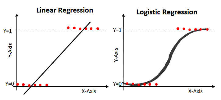
It is used to predict the probability of a dependent variable which is dichotomous (a success or failure state).
It is a modified version of linear regression, which cannot be used as a classification algorithm as its values ranging from infinity to negative infinity, and it returns a continuous value.
These are the types of logistic regression classifications,
-
Binary or Binomial: Dependent variable will only have 2 possible types of either
1(success) or0(failure). - Multinomial: Dependent variable can have 3 or more possible unordered types (e.g. "A", "B" or "C").
- Ordinal: Dependent variable can have 3 or more possible ordered types having a quantitative significance (e.g. "XS" < "S" < "M" < "L").
(Source: Meet Nandu, 2019)
Logistic regression is essentially a modified version of linear regression.
We require the hypothesis function to be in this range .
Therefore to achieve that, we use the Sigmoid function where it is,
Plugging it into the linear regression equation where,
Becomes the hypothesis function,

(Source: StatQuest with Josh Starmer, 2017 - MLE for a seemingly normally distributed data where placing the mean to the center where most data points reside displays the highest "likelihood" value)
To find the value of , we would utilize the Maximum likelihood function (MLE), where the ideal goal is to find the maximum "likelihood" value possible of the parameter(s) value (e.g. standard deviation, weights). The first step is to make an explicit modeling assumption about the type of distribution the data is sampled from, and then set the parameters of the distribution to find the maximum "likelihood" possible value of the parameters.
The likelihood function could be represented as a Bernoulli distribution (is a Binomial distribution with a special case where n=1) as such with parameters (in this case represents the number of data points).
Given that,
Then, given that is the number of success (either
0 or 1 label), is the probability, and there is only 1 trial,
Which gives the likelihood function as,
In short, we want to find the values of that results in the maximum value of the likelihood function. This should result in finding an estimated
and
,
In some cases, we want to regularize the weights to find the optimal weight to prevent overfitting. To do so, we add a regularization function to penalize large weights where,
For L2 type, there is the Ridge regression (L2) where (for dual problem, read here) where,
For L1 type, there is the Lasso regression (L1) where,
For Elasticnet, it is a combination of L1 and L2 where,
- L1 regularization is more complex as the derivative of
is non-continuous at
0. - L2 preferes weight vectors with many small weights, L1 prefers sparse solutions with some larger weights but many more weights set to
0. - L1 regularization leads to much sparser weight vectors and far fewer features.
Imagine the scenario of deducting the weight each time the cost function attempts to find the optimal max weights.

(Source: Machine Learning & My Music, 2019)
For finding the optimized , read here.

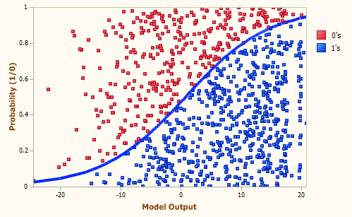
(Source: Ayush Pant, 2019 - Decision boundary at 0.5)
For the hypothesis function to classify between the 2 states 0 or 1, there ought to be a decision boundary of 0.5.
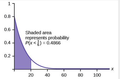
(Source: lumenlearning.com, n.d. - Example of PDF from origin to determine probability)
Given that it is a continuous variable, starting from the origin, the calculation of the probability works like that for the binary classifier,
See how results in the hypothesis function, which is used to determine if the outcome is class
1 (and not means class 0).
As logistic regression at its core is a binary classifier, combinations of this binary classifier are required to handle multi-class cases.
One of them is the One-vs-Rest (OVR) method where a class would be compared against the rest where,
This attempts to find the probability for class for the given
data point.
- There will be
number of classes and the new data point will be classified under the class with the highest vote (or percentage).
- An extra weight specific for each class is
to adjust the percentage for cases where more data points might be larger in some class (imbalance).
- For each class
, its hypothesis function is
.
Using an example of Red, Blue, Green classes, this should create the following combinations,
- Probability of Red: Red vs (Blue and Green)
- Probability of Blue: Blue vs (Red and Green)
- Probability of Green: Green vs (Blue and Red)
To classify the data point to the class, the class with the highest vote (or probability) is chosen.
Another is the One-vs-One (OVO) method where each class is compared against a combination.
Using an example of Red, Blue, Green and Yellow classes, this should create the following combinations,
- Red vs Blue
- Red vs Green
- Red vs Yellow
- Blue vs Yellow
- Blue vs Green
- Green vs Yellow
Hence to classify the data point, choose the highest probability of either,
- Probability of Red: (Red vs Blue) or (Red vs Green)
- Probability of Blue: Inverse(Red vs Blue) or (Blue vs Green)
- Probability of Green: Inverse(Red vs Green) or Inverse(Blue vs Green)
And because it is a regression model, we need to optimize the values accordingly to its cost function, where the cost function for the linear regression is,
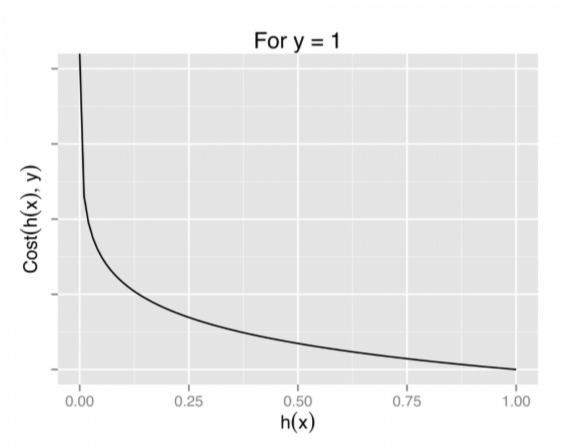
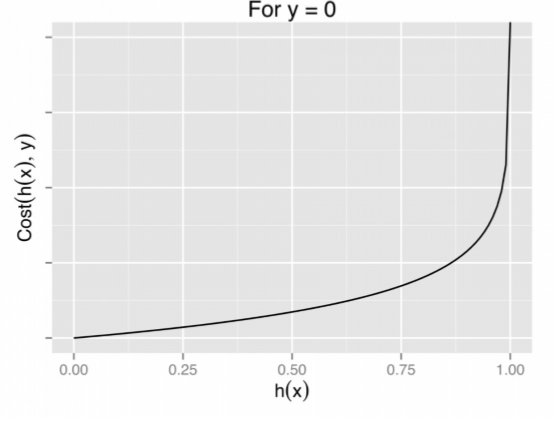
(Source: Ayush Pant, 2019 - To interpret this, for y=0 case, its related hypothesis function returning closer to 1 would mean minimal errors, and closer 0 means a huge room of errors. This is similar conversely for y=1.)
Which in the logistic regression, when being worked out it becomes,
Example algorithms that implement such are Gradient descent algorithm or Newton-CG algorithm.

(Source: fromthegenesis.com, 2018)
K-Nearest Neighbour (KNN) is one of the simplest ML algorithms which assumes the similarity between new data points with the most similar available categories nearest to it. It's a non-parametric algorithm, which means it does not make any assumption on the underlying data and is a lazy learner algorithm since it only starts learning from the training set once a new data point is received.
The drawback of using this algorithm is due to its computation time taken to classify new data points.
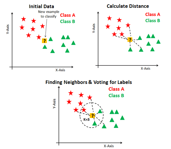
(Source: Avinash Navlani, 2018)
In summary, the algorithm works like this,
- Using a distance algorithm, calculate all the distances between the new point to the other points.
- Re-order all the data points and their distance starting from the smallest to the largest distance.
- Depending on the algorithm used,
- For the 1-nearest neighbor classifier, select the first data point from order.
- Sort the new data point's class from the first data point's class.
- For the weighted nearest neighbour classifier, select first
data points.
- Sort the new data point's class based on the majority voted class
- Sort the new data point's class based on the majority voted class
- For the 1-nearest neighbor classifier, select the first data point from order.
For the weighted algorithm for determining the percentage of votes for each class ,
- The weight algorithm
, depending on the type of mechanism, can be uniform where
or a result based on the distance from the data point to the new data point.
- The
determines if the data point belongs to class
0or1.

(Source: Maarten Grootendorst, 2021)
For the distance algorithm, the Euclidean distance is commonly used (for dimensions and
) where,
Another algorithm is Minkowski distance, which is a generalized format of the Euclidean distance and the Manhattan distance
Where the Manhattan distance is,
And the Minkowski distance is basically (where is
1 or 2 generally),
SVM determines the classes if the data point is >= 1 (upper decision boundary) or (<= -1) (lower decision boundary). This has been covered here.
For multi-class versions, read the multinomial section for OVO and OVR as the same methodologies apply.
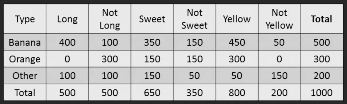
(Source: Selva Prabhakaran, 2018)
Naive Bayes classifier is a simple probabilistic classifier based on applying Bayes theorem. Data sets for each class are fitted into a normal distribution, which would be used later for predictions.
Like the Bayes theorem where,
In summary, the probability can be described in words as,
Bayes’ theorem states the following relationship, given class variable for class
and dependent features (
dimensions) vector
,
Since is a constant given the input, we can approximate to get the following classification rule,
This leads to the Maximum a posterior (MAP) estimation to find the approximate for
(for each class
) such that,

(Source: @108kaushik, 2016)
The formula for the gaussian distribution is that for each class and its feature
, it would have its own gaussian distribution with variance
and mean
.
This is useful for features that have continuous variables such as weight, height.
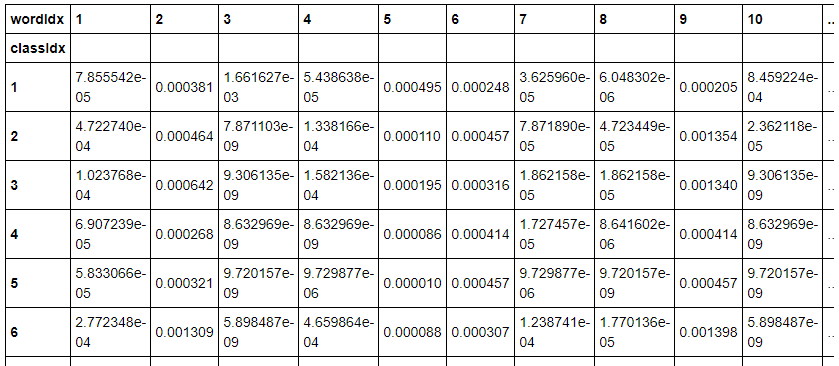
(Source: Syed Sadat Nazrul, 2018)
The formula for multinomial distribution is is that for each class and its feature
, it would have its own multinomial distribution.
Where the total number of features. This is useful for features that have countable discrete variables such as the number of boys and girls in a team.

(Source: THEAGATETEAM, 2020)
The formula for bernoulli distribution is is that for each class and its feature
, it would have its own bernoulli distribution.
This is useful for features that have boolean variables such as yes/no or success/failure.
Similar to the Decision Tree Regression algorithmic steps except for the difference in metrics and algorithm used.
For the CART algorithm, it uses the Gini's Impurity metric to determine the split and its branches (uses Eucleadian distance to calculuate distance).
In summary, it attempts to find the minimum Gini impurity, where the lesser the amount, the less variance in the branch's data set. The final (or terminal) node should be the class label to which the new data point would be classified.
- The sets of data points are
which represents the total in the current branch (or node), and
(left) and
(right) the total in the partitions.
-
represents a class in
-
represents the total number of data points in
and
respectively).
-
and
represents their weighted component respectively, where it is the proprotion of the left and right split (e.g. weighted number of samples in each partition over the number of samples in the node).
(Source: Andre Ye, 2020)
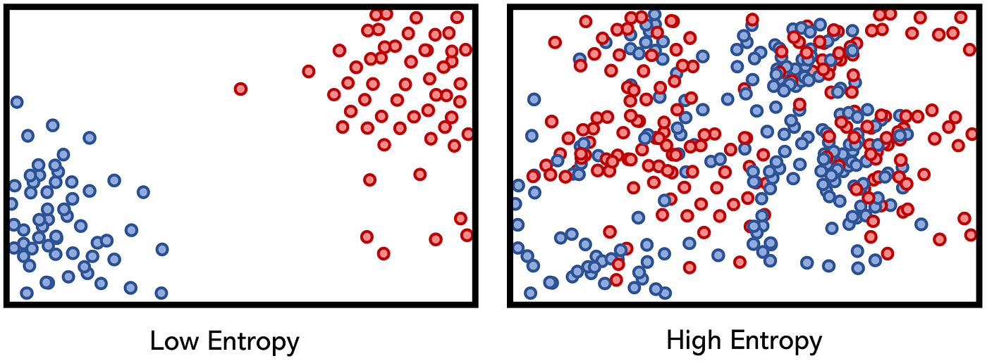
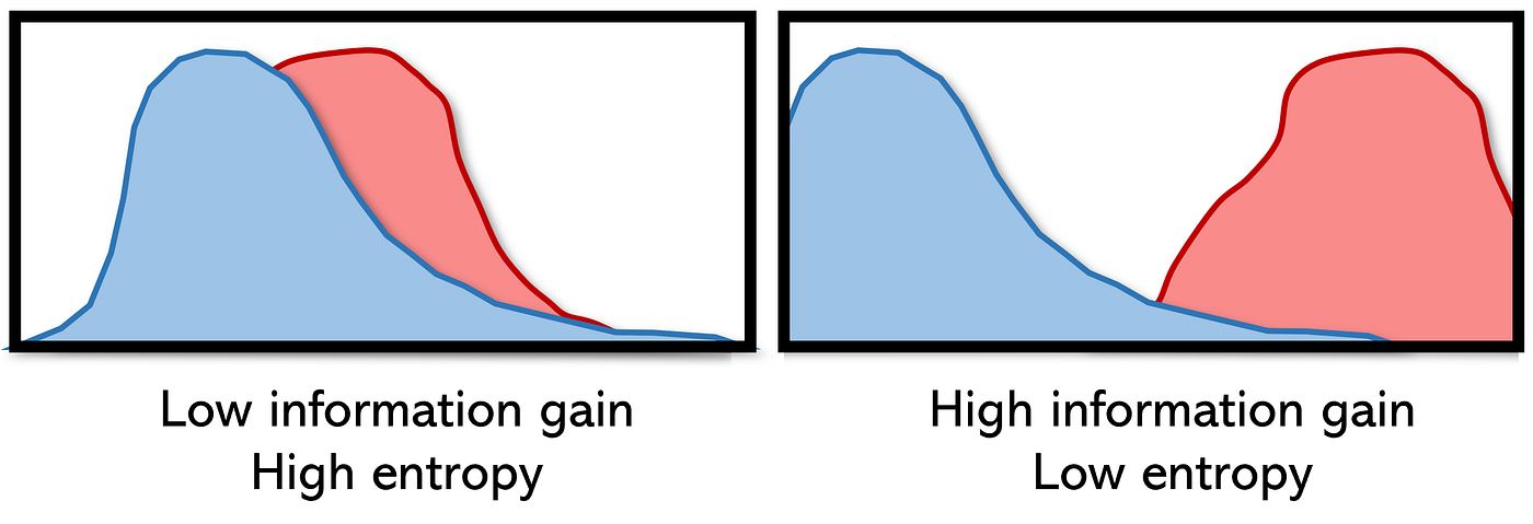
Entropy is the measure of disorder or uncertainty, for decision trees, the goal is to reduce entropy when determining branches in its split so that a more accurate prediction can be done. Information gain is the reduction in entropy or surprise by transforming a dataset.

(Source: Andre Ye, 2020)
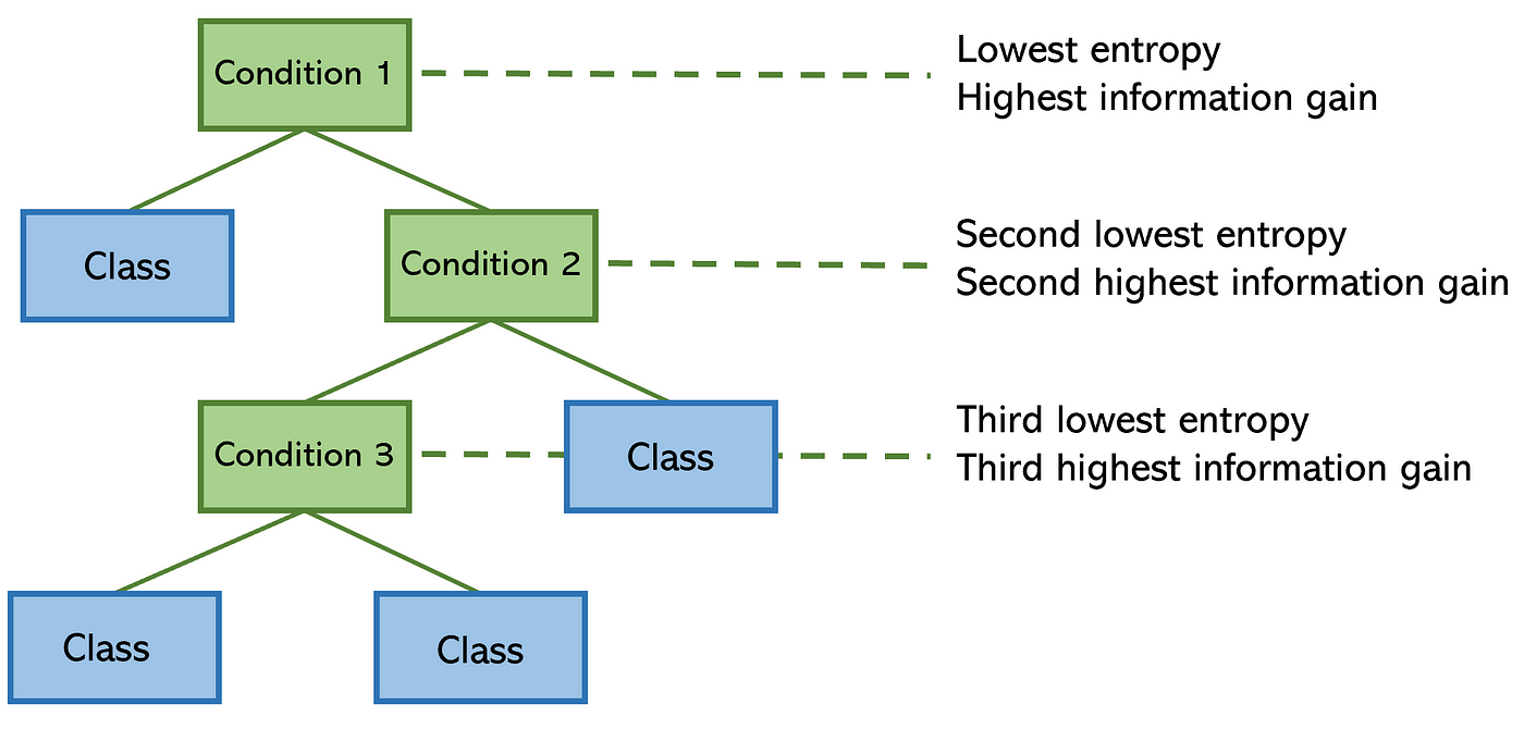
For the ID3 algorithm, it uses Information Gain (IG) to determine the split and its branches (uses Eucleadian distance to calculate distance). The one with the highest IG would be chosen to become the next branch to split from.
This calculates how much entropy has been removed by using IG (which is the result in the set). Similarly, the final (or terminal) node should be the class label to which the new data point would be classified.
Feature importance is the decrease in node impurity weighted by the probability of reaching the node. The higher the value the more important the feature.
-
calculates the number of splits for the feature.
-
represents the number of features in the training data set
.
Similar to the Random forest regression except the majority vote classifies the new data point.