In this tutorial, we will train and evaluate multiple time-series forecasting models using the Store Item Demand Forecasting Challenge dataset from Kaggle. This dataset has 10 different stores and each store has 50 items, i.e. total of 500 daily level time series data for five years (2013–2017).
- Download the train.csv from https://www.kaggle.com/competitions/demand-forecasting-kernels-only/data?select=train.csv.
- Create a
./datadirectory inside the directory of this Python notebook - Save the train.csv inside the
./datadirectory
| date | store | item | sales | |
|---|---|---|---|---|
| 0 | 2013-01-01 | 1 | 1 | 13 |
| 1 | 2013-01-02 | 1 | 1 | 11 |
| 2 | 2013-01-03 | 1 | 1 | 14 |
| 3 | 2013-01-04 | 1 | 1 | 13 |
| 4 | 2013-01-05 | 1 | 1 | 10 |
The dataset has 913000 rows and 4 columns
- date - Date of the sale data. There are no holiday effects or store closures.
- store - Store ID
- item - Item ID
- sales - Number of items sold at a particular store on a particular date.


The ACF presents a spike at x in [1, 7, 14, 21], which suggests a weekly seasonality trend (highlighted). The blue zone determines the significance of the statistics for a confidence level of m.
# Import necessary models from the statsforecast library
from statsforecast.models import (
    # SeasonalNaive: A model that uses the previous season's data as the forecast
    SeasonalNaive,
    # Naive: A simple model that uses the last observed value as the forecast
    Naive,
    # HistoricAverage: This model uses the average of all historical data as the forecast
    HistoricAverage,
    # CrostonOptimized: A model specifically designed for intermittent demand forecasting
    CrostonOptimized,
    # ADIDA: Adaptive combination of Intermittent Demand Approaches, a model designed for intermittent demand
    ADIDA,
    # IMAPA: Intermittent Multiplicative AutoRegressive Average, a model for intermittent series that incorporates autocorrelation
    IMAPA,
    # AutoETS: Automated Exponential Smoothing model that automatically selects the best Exponential Smoothing model based on AIC
    AutoETS
)# Import the necessary models from various libraries
# LGBMRegressor: A gradient boosting framework that uses tree-based learning algorithms from the LightGBM library
from lightgbm import LGBMRegressor
# XGBRegressor: A gradient boosting regressor model from the XGBoost library
from xgboost import XGBRegressor
# LinearRegression: A simple linear regression model from the scikit-learn library
from sklearn.linear_model import LinearRegression


XGBRegressor was the best performing model based on MSE for 2 out of the 3 validation folds of store_item 1_1.

LGBMRegressor was the best performing model based on MSE for 2 out of the 3 validation folds of store_item 1_1.


This code is based on the following publicly available resources
- Nixtla Statistical, Machine Learning and Neural Forecasting methods
- Intro to Forecasting with Darts
- Store Item Demand Forecasting Challenge dataset from Kaggle
Part 2 - Multiple Timeseries Forecasting with Covariates - Cracking the Code 👩💻📈 Predicting Crypto Prices with Multiple TimeSeries and Covariates
Use time series forecasting models with covariates ('Days Until Bitcoin Halving', 'Fear & Greed Index') to predict crypto prices (BTC, ETH, DOT, MATIC, SOL).
Our objective is to employ the training series for forecasting cryptocurrency prices within the validation series, assess model accuracy through metrics, and determine the best-performing model for the task at hand.
In part two we discuss how to:
- Add covariates to your timeseries forecasting model
- Backvalidate model predictions
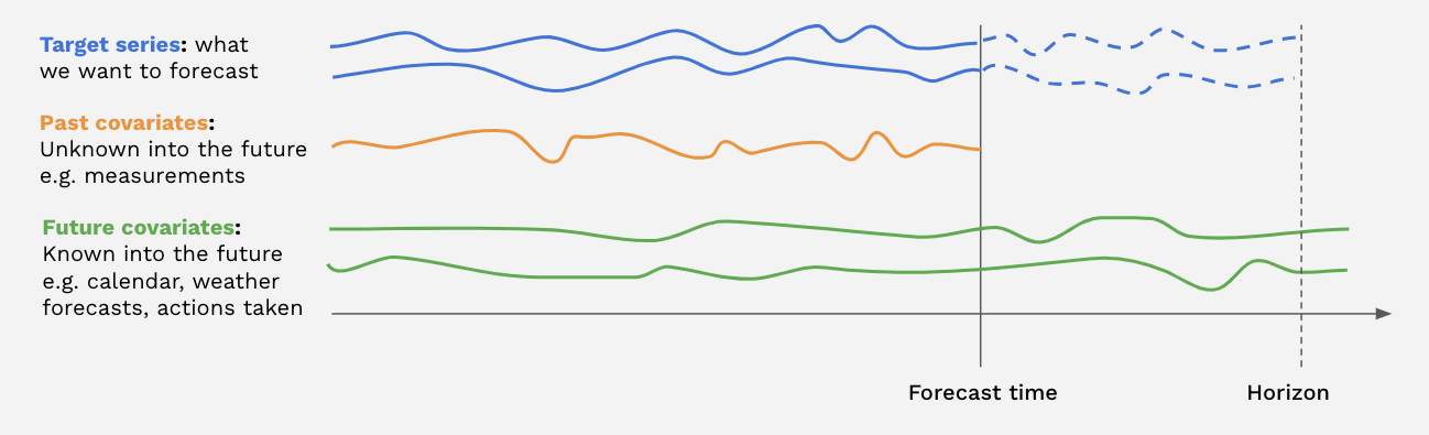
In addition to the target series (the series we aim to forecast), many models in Darts also accept covariate series as input.
Covariates are series that we don't intend to predict but can offer valuable supplementary information to the models. Both targets and covariates can be either multivariate or univariate.
There are two types of covariate time series in Darts:
past_covariatesconsist of series that may not be known in advance of the forecast time. These can, for example, represent variables that need to be measured and aren't known ahead of time. Models don't use future values of past_covariates when making predictions.future_covariatesinclude series that are known in advance, up to the forecast horizon. These can encompass information like calendar data, holidays, weather forecasts, and more. Models capable of handling future_covariates consider future values (up to the forecast horizon) when making predictions.
Each covariate can potentially be multivariate. If you have multiple covariate series (e.g., month and year values), you should use stack() or concatenate() to combine them into a multivariate series.
In the following cells, we use the darts.utils.timeseries_generation.datetime_attribute_timeseries() function to generate series containing month and year values. We then concatenate() these series along the "component" axis to create a covariate series with two components (month and year) for each target series. For simplicity, we directly scale the month and year values to a range of approximately 0 to 1.

The historical_forecasts feature in Darts assesses how a time series model would have performed in the past by generating and comparing predictions to actual data. Here's how it works:
- Model Training: Train your time series forecasting model using historical data.
- Historical Forecasts: Use the function to create step-by-step forecasts for a historical period preceding the training data.
- Comparison: Compare historical forecasts to actual values from that period.
- Performance Evaluation: Apply metrics like MSE, RMSE, or MAE for quantitative assessment.
- Insights and Refinement: Analyze the results to gain insights and improve the model.
This process is essential for validating a model's historical performance, testing different strategies, and building confidence in its accuracy before real-time use.
