Network modelling of stereotactic EEG data

work in progress | About this research stream | ICTALS2017 Poster

This repository contains the code required to reproduce a network based approach to SEEG data analysis that aims to simulate epilepsy surgery in silico to help improve surgical planning in the future. This project is work in progress and has not yet been validated for prospective clinical use. The strategy demonstrated here rests on three broad approahces

1. Using nonnegative matrix factorisation (an idea stolen from Chai et al. 2017) to easily visualise network edge dynamics during seizures in a patient undergoing presurgical evaluation for epilepsy surgery using stereotactic EEG.
2. Using hierarchical dynamic causal modelling (parametric empirical Bayesian DCM, which rests on Friston et al. 2016) to identify biophysical network changes that best explain seizure onset across a number of different seizure types within the same patient.
3. Using simulations of fully fitted neural mass models (the output of the DCM analysis) to quantify the effects of in silico node resection on whole network activity

The code runs on Matlab (tested with 2016b) and requires the following freely available packages to run

• Statistical Parametric Mapping, SPM12 - The neuroimaging analysis suite that contains the DCM tools

Table of Contents

1. Custom routines
   1. Visualise Network
   2. Nonnegative Matrix Decomposition
   3. Subnetwork Channels
   4. MEEG Object Filemaker
   5. Grand Mean DCM
   6. DCMs of seizures
   7. Parametric Empirical Bayes
   8. Simulated Surgery
2. [SPM Modifications]
3. [Other Helper Functions]

Custom routines included in this repository

The repository includes a number of custom routines that when run sequentially should reproduce our analysis.

Visualise dynamic network patterns

seeg_networkvis

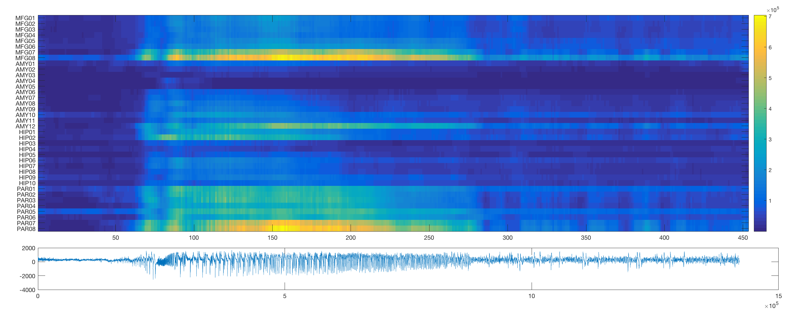
In order to first visualise the network dynamics during seizures in this dataset, this routine plots some of the activity. The first section plots individual channels for the duraction of the seizure activity.

The routine then employs a sliding window approach to estimate the changing output spectral distribution at each channel over time (note that the sliding window in its current implementation will take a long time).

The routine also plots example adjacency matrices derived from windowed coherence and correlation estimates for a pre-seizure and seizure segment in the data.

To track the full temporal resolution of these changes, we can vectorise the adjacency matrix (using the matlab inbuilt function tril to preserve just the unique edges) and plot the resultant vectors for each time window. Note that for better visibility, this routine orders the edges according to their overall mean correlation/coherence.

Run nonnegative matrix decomposition to identify subgraphs

seeg_decomp

This routine will load all available data, concatenate their windowes coherence estimates into a single edge by time matrix, and then decompose that matrix into subgraphs using nonnegative matrix decomposition. This decomposition requires a few different parameters - most importantly the number of subnetworks component into which the data is meant to be decomposed.

This can be chosen to achieve an arbitrary accuracy threshold, and the code will identify the minimum number of subnetworks required to reproduce the data with a +90% accuracy, providing the following visual output.

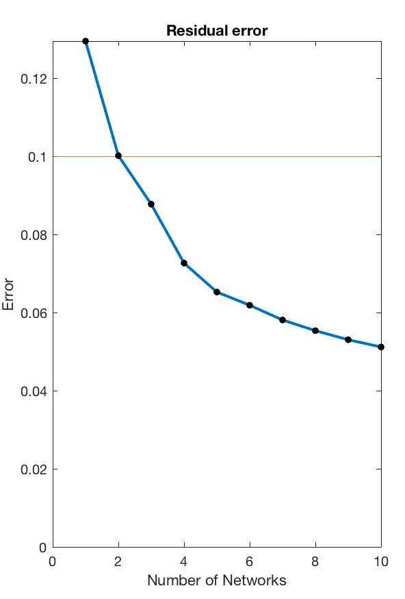
For this particular use case the minimum number of subnetworks is k=3 and the subsequent analysis will be performed using three subnetworks. These are visualised in the next step - both as adjacency matrices (as they are fully weighted), and as a medium-connection-strength thresholded graph representation for visualisation purposes.

We then use the time courses of the different network expressions to identify time points that are associated with the maximum rate of change. For this we can calcualte the sum of the differentials of each time course and place and arbitrary threshold, which we select to identify the time windows containing the biggest change. A time window prior- and after this maximum change will be analysed further using the DCM appraoch.

Identifying a subnetwork of representative channels

seeg_components

In order to keep the DCM analysis at a computationally tractable level of complexity, we need to select a subsection of channels that can be modelled. There are several ways to do this, and this solution here presents a simple approach that aims to (1) select original data channels so that the time series remain interpretable as raw EEG data, and (2) make the selection data-driven and automatic.

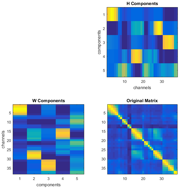
For this we use the same matrix-decomposition algorithm as above, only this time we use it on a symmetrical weighted adjacency matrix derived from coherence across all data points. This decomposition will give us two (very similar) n by k matrices, where n is the number of channels, and k is the number of components. Here we set the components to be identical to the number of SEEG electrodes in the original recording (i.e. 5), which produces the following results:

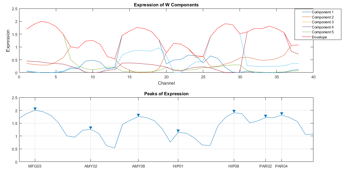
We can plot these components on top of each other and identify regional maxima in the expression of specific components. These correspond to individual channels, and based on these peaks we select a small number of channels that are included in the subsequent DCM analysis. Note that this approach yields 7 peaks from the 5 components, which are included for further analysis in the DCM.

Prepare files for DCM analysis (SPM: MEEG object)

seeg_filemaker

SPM-based analyses use electrophysiological data in a specific matlab object category called the MEEG object. This routine creates two MEEG objects for use in the subsequent DCM analysis, which contains the data in two different ways

1. Multichannel segmented into sliding window, so that each 'trial' in the MEEG-object corresponds to a separate 30s window in the original, concatenated data. This will be used to perform window-of-interest DCM analysis.
2. Single channel concatenated data, so that each 'trial' in the MEEG-object corresponds to a separate channel from the 7-channel selection chosen for DCM analysis. This will be used in the Grand Mean DCM analysis.

The screenshot below shows the first (multichannel, windowed) MEEG object when seen in SPM (open in matlab by calling spm eeg, then select M/EEG from the 'Display' drop down menu.

Run grand mean DCM to specify prior parameter estimates

seeg_gmdcm

Prior parameters for the biophysical models used in SPM are based on cortical columns in healthy human cortex, and are specifically designed to cope well with ERP experiments and particular steady state applications. Here we need to adapt the priors to allow the inversion of abnormal dynamics as seen in epilepsy.

In order to find suitable sections of parameter space, we therefore employ a staged approach to the model inversion

1. Manually set a small selection of parameters to values that are compatible with the spectral output seen in the data
2. Use this parametersiation to invert continuous data from individual channels, yielding a single, 'steady-state' neural mass model parameterisation that reproduces the type of spectral output seen in this particular channel
3. Use the channel-specific parameterisations as priors for further DCM analysis of multichannel networks identifying changes

The first two points are addressed in this routine. Runningspm_induced_optimise allows visualisation of individual parameters' effects on te spectral output of individual model nodes. Based on this, a single parameter (the time constant T(2)) was altered. With the thus adapted priors, this routine runs an inversion for each channel individually. The empirical estimates for the individual channels is then saved for use as priors in the next steps of the analysis.

Run DCM on regions of interest identified from Nonnegative Matrix Decomposition

seeg_dcm

Based on the empirical estimates of region-specific coupling parameters derived from the grand mean DCMs, we then invert a single multi-channel (7 node) DCM for each of the time windows of interest - that is 1 pre-seizure, and 1 established-seizure window for each of the three seizures in question.

The inverted DCMs will encode the differences in the regional activity, and coupling between regions (i.e. their cross-spectral densities) between these time windows in terms of biophysical parameters of a neural mass model. This is a reasonably time consuming step.

Run hierarchical parametric empirical model to identify seizure-related model changes

seeg_peb

After inverting DCMs individually for the pre-seizure and within-seizure time windows, we use parametric empirical Bayesian modelling to identify across-DCMs effects that are consistently induced by seizures. These are then plotted as networks of varying between-source connectivity (i.e. edge modulation) and varying degrees of intrinsic self-inhibition (i.e. node modulation) as in the example shown below.

Simulate surgical interventions and quantify network effects

seeg_surgery

In order to simulate the effects of surgical removal of individual areas, we simulated surgery based on the models that were parameterised using the DCM approach. To simulate resection of individual areas, we removed all connection from this area and then simulated the steady state model output, leaving all other parameters unchanged.

The output of this function is a (maximum-normalised) plot of the difference induced by the in silico surgical intervention on the first principal eigenmode power spectrum and coherence to capture both amplitude and phase effects.