6. Creating a map
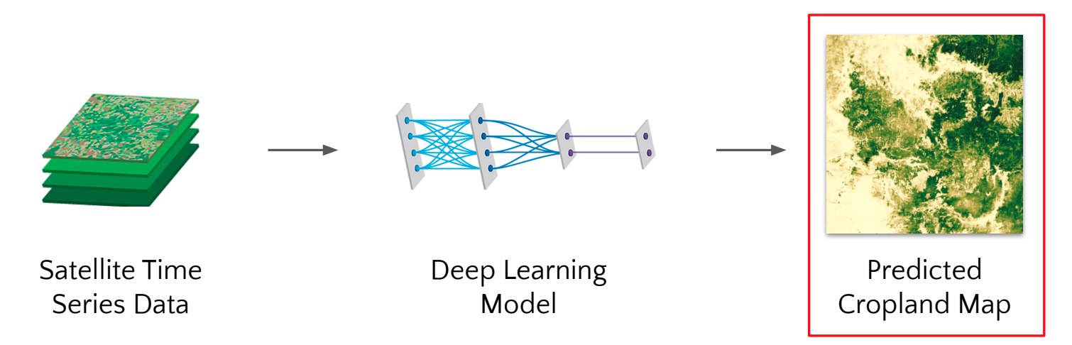
The following instructions will guide you through generating a cropland map using a trained model.
Prerequisite: Model Training
- Inside the notebook, you will be required to paste the content of your
openmapflow.yaml(also known as the project configuration file). To locate your project'sopenmapflow.yaml, check yourcrop-maskrepository. And paste it into the widget prompt. Theyamlfile contents are essential to make the package workflow seamless. - Authenticate both Google Cloud and Earth Engine to current your account to the runtime.
- Then run the cell with
!gcloud run service list ....; this fetches the trained models that were already deployed from theModel Trainingstep.
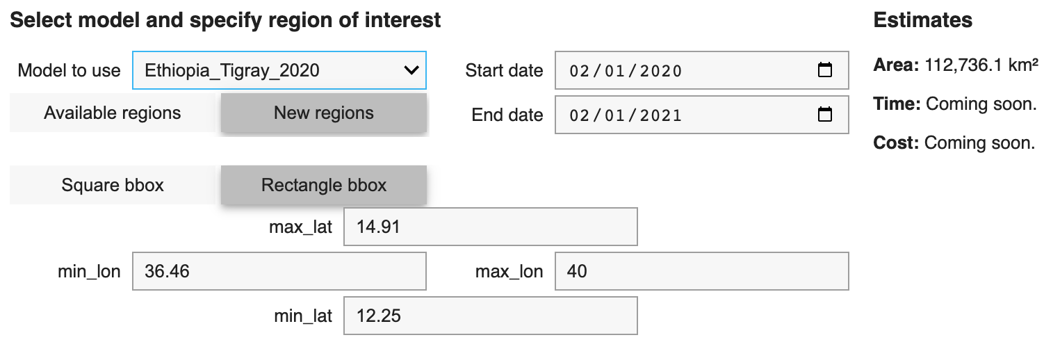
There are a few things needed when configuring the inference:
- Trained model,
- start and end date of the trained model, which is the map year to create. (e.g. 02/01/2020 to 02/01/2021),
- and the map's region of interest (ROI) to create.
Note: The New regions button is used when configuring an ROI for the first time. Subsequently, the ROI configuration will be added to the Available regions once the inference run is completed.
- Run the cell with
available_bboxes = get_available_bboxes(); to get the regions we already have their Earth observation data stored. - Run the
inference_widgetfor configuration- Select the model to use in the dropdown,
- Select the start and end date.
An easy way to define a region of interest is using a bbox (either square or rectangle) as specified in the inference widget. You can get a bbox (i.e. lat, lon or min_lat, min_lon, max_lat and max_lon) using bboxfinder.com.
Note: Defining region of interest using country administrative boundary (coming soon).
- Run the following cell, which gets your configuration details into specific variables and check if there is an existing map file in the cloud storage with the same configuration; if this is the case, you will be prompted to add a version id.
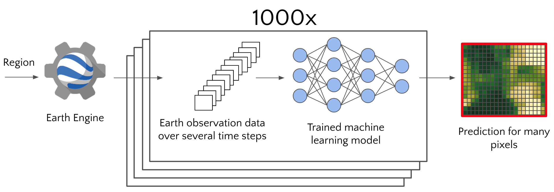
The next process made dense inference easy by cloud computing using thousands of optimized trained models deployed on the Google Cloud Run service to predict thousands/millions of imagery pixels rapidly.
-
Run the
inference_statuscell.
A short description of what is going on here:
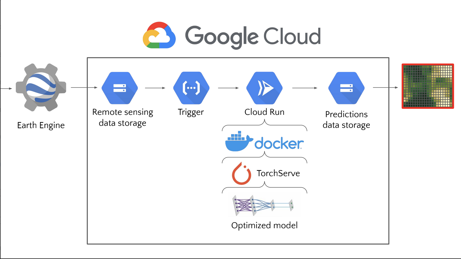
The Openmapflow Google Cloud architecture in the image above facilitates rapid predictions. A brief description of each component:
- Running the
inference_statuscell activates the export of Earth observation data from Earth Engine according to the inference configuration (within the ROI and time range) into the cloud data storage, - this export process triggers some Cloud functions and the Cloud Run service in which an optimized model is packaged in a TorchServe and a Docker container. The Cloud Run service multiplies the Docker container into thousands based on the number of data available for inference,
- once the Cloud Run makes the prediction, they are saved in the prediction data storage.
Monitor Earth Engine exports progress here.
This process might take minutes or hours, depending on the extent of the ROI.
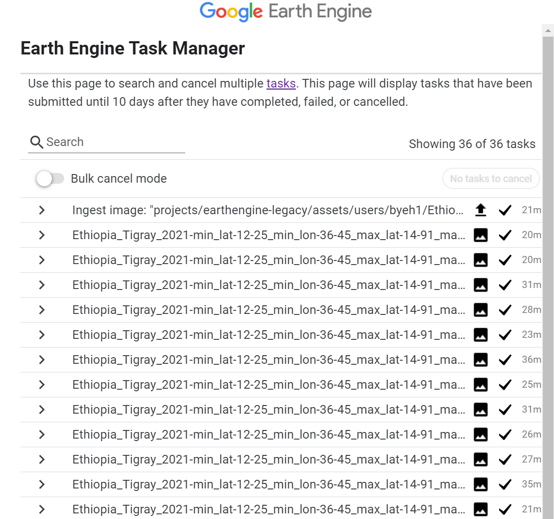
Once the Earth Engine export completes, re-run the Inference_status cell to check the progress on the prediction made.
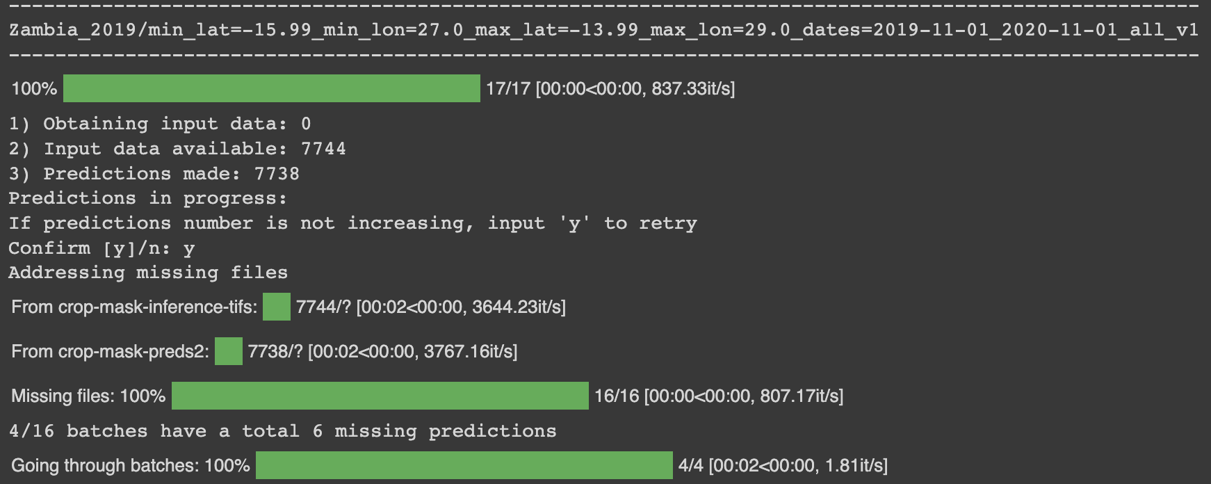
Note:
- Obtaining input data: The amount of data to be exported by Earth Engine,
- Input data available: Amount of data available for prediction,
- Prediction made: Amount of prediction data.
The amount of prediction made should equal the available data for prediction; therefore, the cell is run multiple times to ensure both are equal.
There are special cases when both numbers do not equal; this might be due to several issues. Therefore, tracking the inference logging on gcloud console is needed. This only gives an insight into what might be the cause.
The predictions made are stored in the cloud storage bucket specified in bucket_preds of the openmapflow.yaml file.
The merging process includes the following:
- Download predictions files from the cloud bucket
- merge using GDAL
- upload the merged map into the specified merge bucket
bucket_preds_merged, - upload as Earth Engine asset
When creating a large map, merging on a computer/virtual machine with bigger memory space is advised using this script.
- Earth Engine: https://earthengine.google.com/
- Cloud Run Service: https://cloud.google.com/run/docs/overview/what-is-cloud-run
- TorchServe: https://pytorch.org/serve/
- Docker:https://docker-curriculum.com/