This project thesis aims to implement an Anomaly Detection framework using a Self-Supervised approach.
Self-supervised learning (SSL) is a subcategory of unsupervised learning. This method can achieve an excellent performance comparable to the fully-supervised baselines in several challenging tasks such as visual representation learning, object detection, and natural language processing.
SSL learns a generalizable representation from unlabelled data by solving a supervised proxy task (called PRETEXT TASK) which is often unrelated to the target task, but can help the network to learn a better representation.
Pretext task examples:
- Rotation classification
- jigsaw puzzle
- denoising
The Pretext Task is solved creating an artificial dataset based on the original unlabelled dataset, where the model is trained to solve a problem in a supervised approach using pseudo labels (autogenerated during the dataset preparation, no human manual labeling).
After training the network, the knowledge (weights) are transferred in a new model (equal or smaller) to solve the so-called Downstream Task (the original problem we wanted to solve), using the original real data.
For the pretext task an artificially created dataset is used. It consists of three classes of elements (image without defects, image with large transformation, image with small transformation). The generation and labeling phase is performed automatically at runtime: during training, for each image in the batch, a random value Y (the label associated with the image) is first generated in the interval [0, 2].
If the value of Y is greater than zero the image is transformed to generate the error. Errors are entered by means of geometric transformations. If the generated label Y is 0, then only basic augmentation transformations such as Contrast, Brightness, and Hue are applied to the image.
The artificial defects can be a cut-paste of a portion of the image, an average color or a flat random color.
If the Y label is equal to 1, a non-regular polygon is generated within the image. To create the polygon a randomly sized rectangle is first defined taking into account area_ratio and aspect_ratio.
area_ratio refers to the ratio of the area of the rectangle in question to the total area of the image. It is a real value randomly chosen in the interval [0.03, 0.1] (for patch-level localization in [0.1, 0.2]).
aspect_ratio refers to the ratio of the length to the height of the rectangle, and is a randomly chosen value in [0.3, 1)U(1, 3.3].
Having length and height of the rectangle, a region of the image is cut within 4 random points (a,b,c,d)
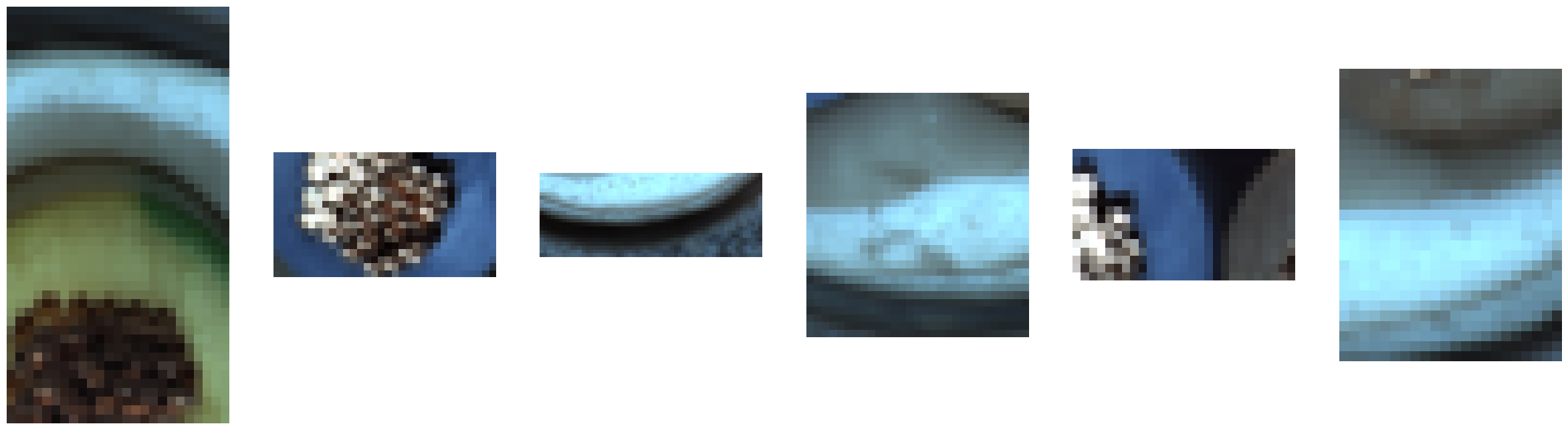
If the element in question is a texture (for example carpet), the cut is done by taking an image of a random element in the mvtec dataset (for example a portion from an image of the bottle object is taken). This is to avoid that the cut part, once pasted on the original image, gets confused too much with it.
Since carrying out cutting operations to obtain non-regular polygons could be complicated, the idea is to construct a binary mask of the aforementioned polygon, to be subsequently applied on the rectangle just obtained. For each side of the rectangle, 1 or 2 points are chosen, thus obtaining a polygon with a minimum of 4 sides and a maximum of 8. The points are generated in such a way that the polygon is convex.
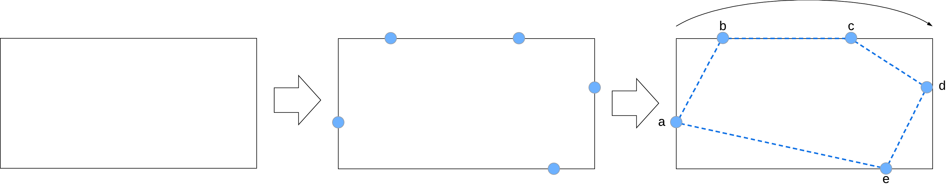
The mask is generated such that the pixels are equal to 0 if outside the polygon, 1 otherwise.
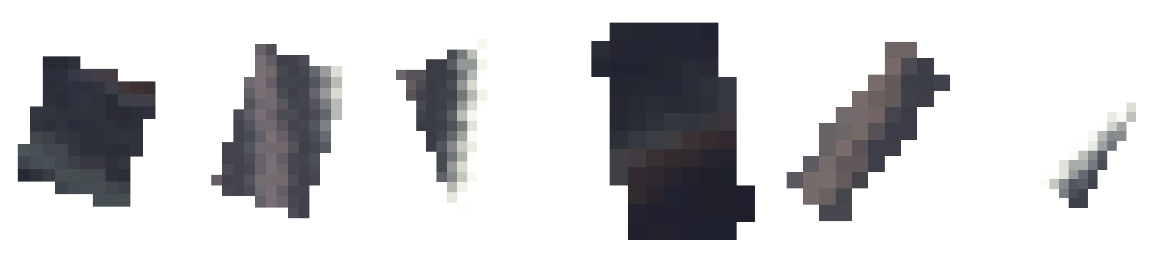
If the Y label equals 2, a line is generated within the image. The line is a small randomly generated rectangle similar to the large defect, with the difference that area_ratio and aspect_ratio are respectively [0.003, 0.007] and [0.05, 0.5)U(2.5, 3.3] (in patch-level area_ratio is [0.01, 0.02]).
The extracted rectangle is then rotated within a range of [-45, 45] degrees.
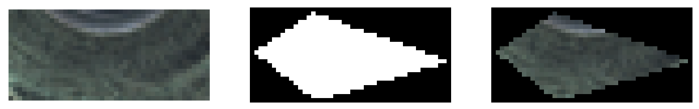
To make artificial defects more realistic, it is fair to think that they must be inside the object in question. Before proceeding with the generation of the defects, a binary mask of the image is built, which represents the object present inside it (in the case of textures, the mask will have all the positive pixels). In the case of objects with fixed position and texture, the mask is built only once for the entire duration of the training, this is justified by the fact of lightening the computational cost.

A set of coordinates is extracted from the mask, from which a pair (x,y) is then randomly taken. The couple represents the center of the artificial defect.

The architecture of the network is structured as follows: a ResNet-18 is taken as the backbone, suitably modified to also use the intermediate outputs of convolutional blocks 2 and 3. The backbone is followed by a fully-connected which takes care of both concatenating layer2, layer3, layer4 outputs and reduce the number of features. Then there is a projection head, a series of fully-connected to process the features and obtain them in the form of a linear vector. The output of the projection head is connected to a classifier during the pretext task, otherwise to an anomaly detector, where given an input vector the cosine similarity is calculated with a vector of features representing the "normality", subsequently returning an anomaly score in [0,1].
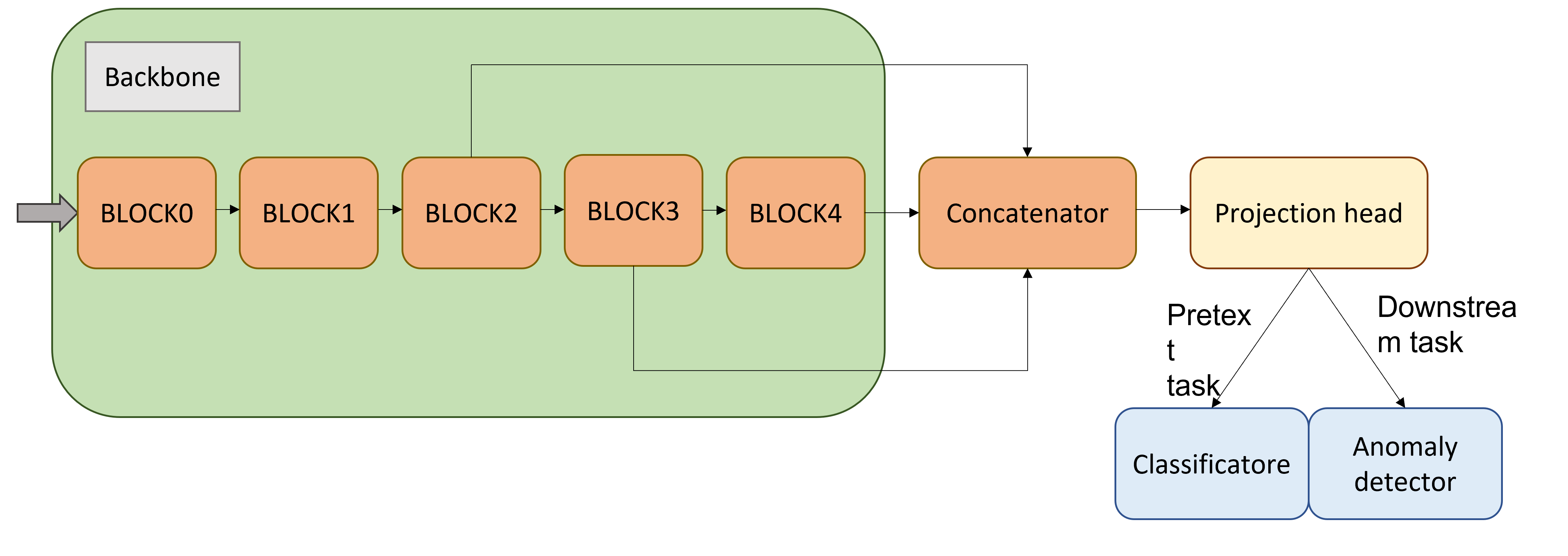
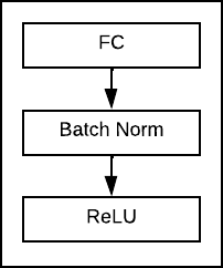
Each block of the projection head is composed of a fully connected, a batch normalization and a ReLU function.
One model is trained for each element class of the MVTec dataset (15 models in total).
The backbone is loaded with imagenet weights.
Each model is trained on epochs=10 with learning_rate=0.03, only changing the projection head weights.
Then a training is done unlocking the whole network with epochs=50 and learning_rate=0.01. The optimizer used is SGD with momentum=0.9, with weight_decay=0.0005, on which a Learning Rate Scheduler (Cosine Annealing Schedule) is subsequently applied.
A batch_size=96 is used and since the training data are few (about 200/300 images per mvtec element), they are duplicated to obtain a minimum of 500 filenames.
During the training phase a memory bank is used. The purpose of the memory bank is to memorize the embedding vectors representing the normal data. During the training step, for each batch the embedding vectors with label y=0 and predicted with y_hat=0 are filtered and inserted into the memory bank. At the end of each epoch the excess data in the memory bank are eliminated, discarding the oldest ones.
To perform a patch-level and not image-level approach, before applying geometric transformations to the images, they are randomly cropped with a patch_size=32.
In the inference phase, the embedding vector of an image is extracted and subsequently given as input to an Anomaly Detector. The anomaly score is calculated by evaluating the average distance between the edging vector and 3 vectors considered "normal", taken from the memory bank with the Nearest Neighbor approach. The metric for distance is Cosine Similarity.
For the patch-level approach, the test image is decomposed into small patches with patch_size=32 and with stride=8.
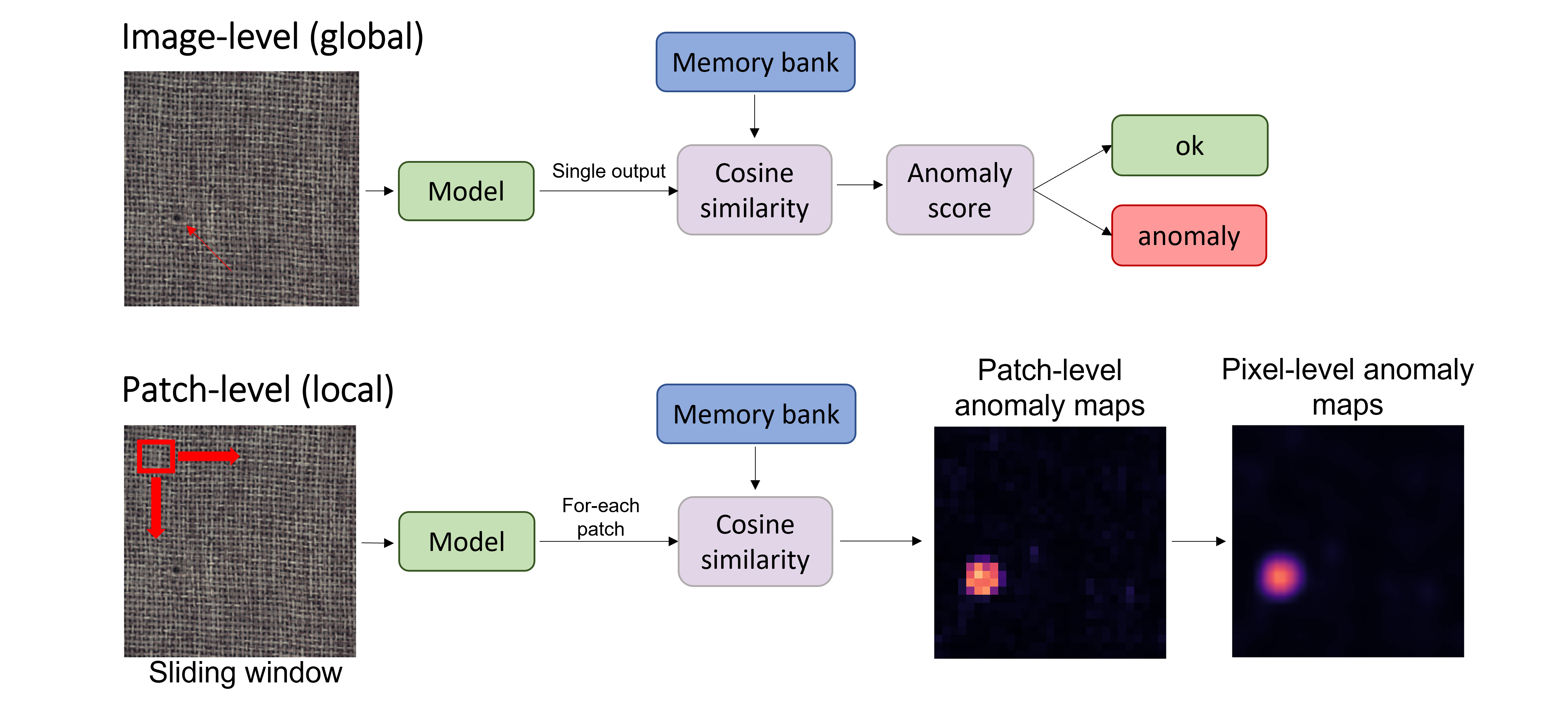
For the image-level approach the GradCam is used to obtain an anomaly map relating to a test image. For the patch-level approach, an embedding vector is extracted for each patch and its anomaly score calculated, as presented previously. Subsequently an upsampling with bilinear interpolation is done to obtain an anomaly map of dimensions equal to the test image.
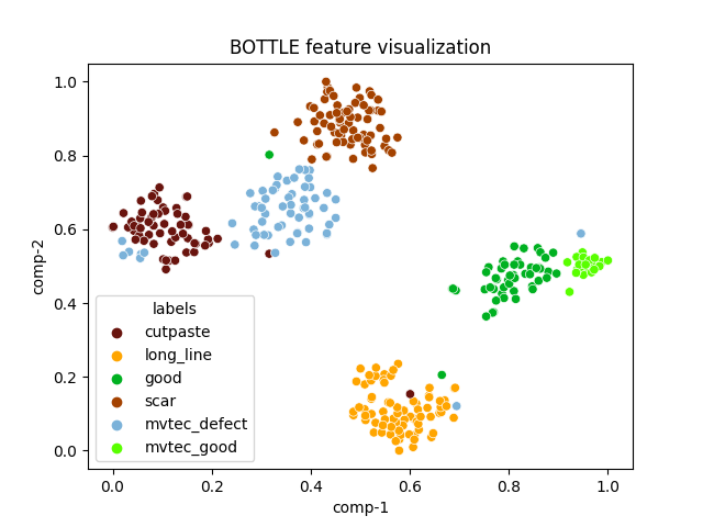
| roc (classification image level) | roc (localization patch level) | tsne | |
| bottle |  |
|
 |
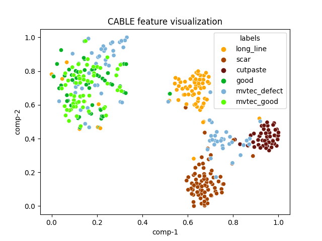
| cable | 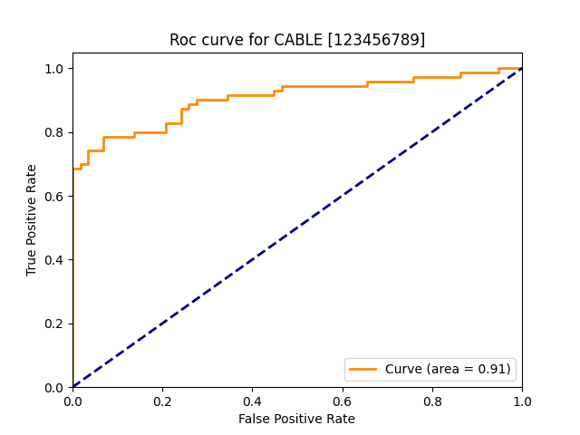 |
|
 |
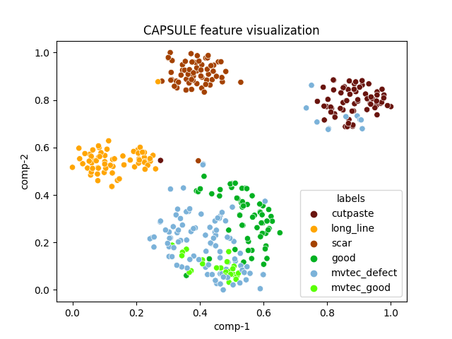
| capsule |  |
|
 |
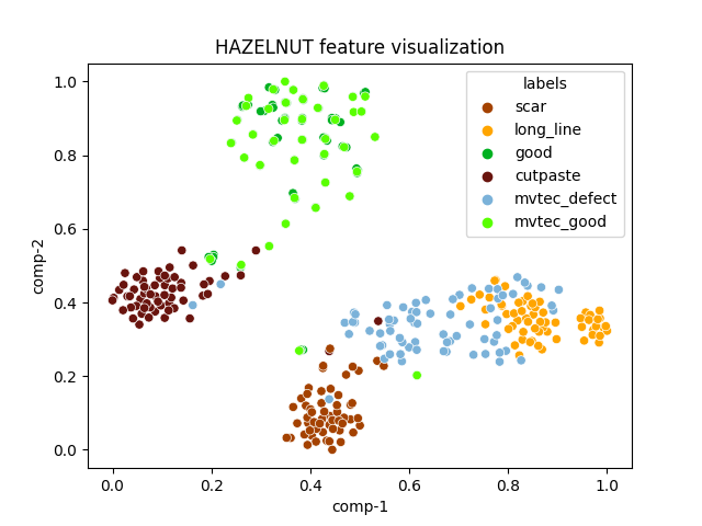
| hazelnut | 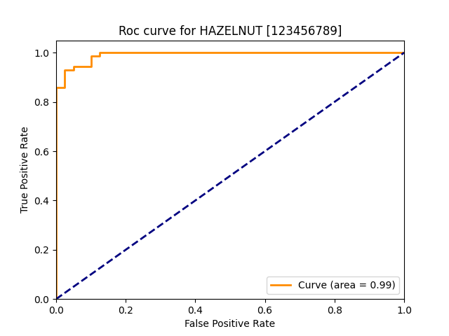 |
|
 |
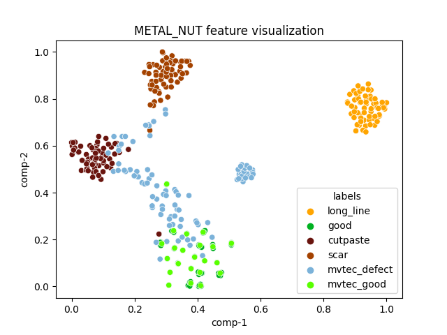
| metal_nut | 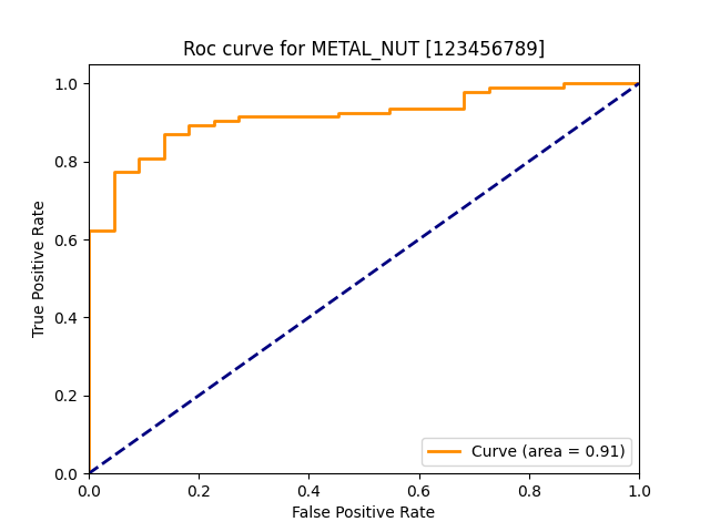 |
|
 |
| roc (classification image level) | roc (localization patch level) | tsne | |
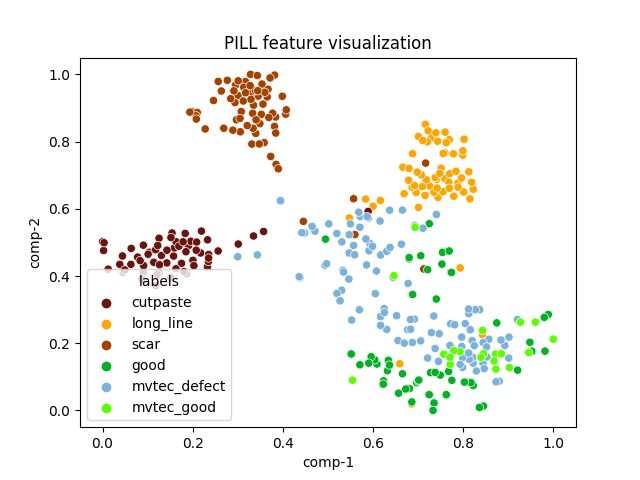
| pill | 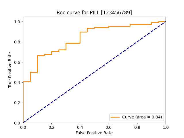 |
|
 |
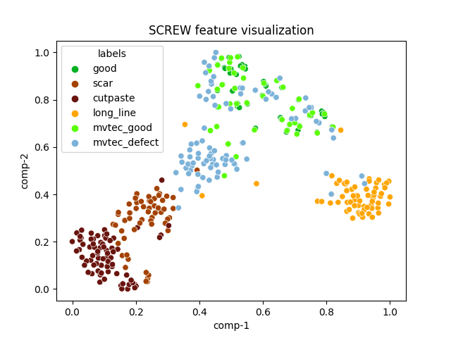
| screw | 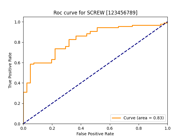 |
|
 |
| toothbrush |  |
|
 |
| transistor | 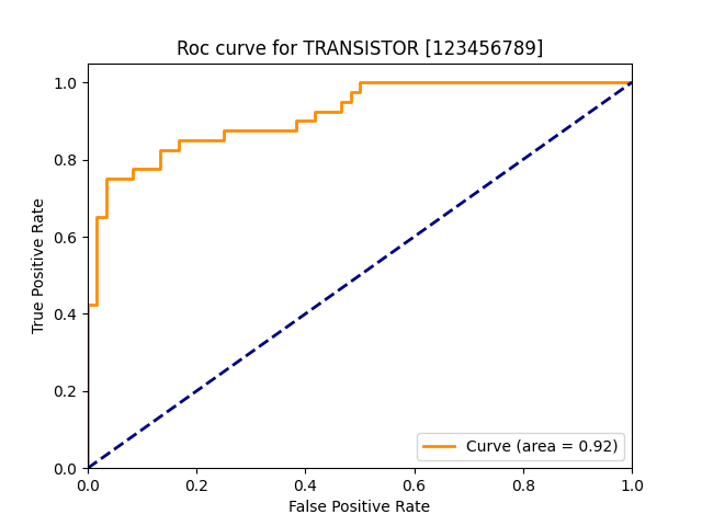 |
|
|
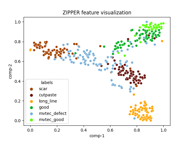
| zipper |  |
|
 |
| roc (classification image level) | roc (localization patch level) | tsne | |
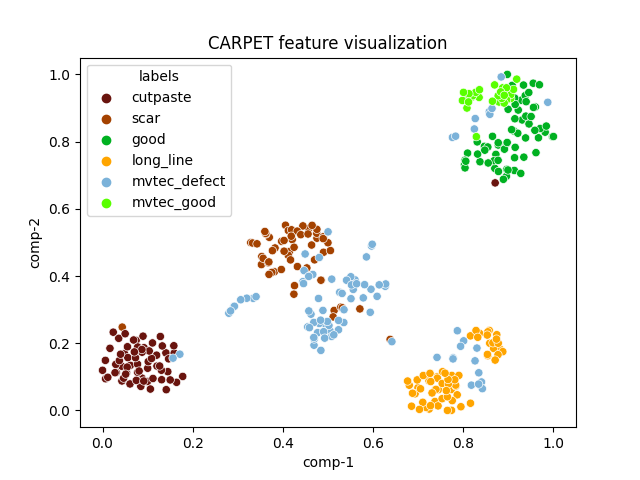
| carpet | 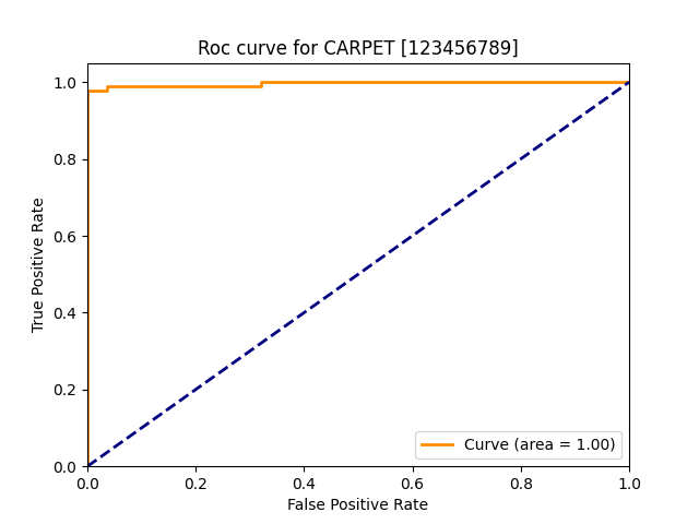 |
|
 |
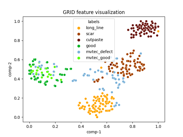
| grid | 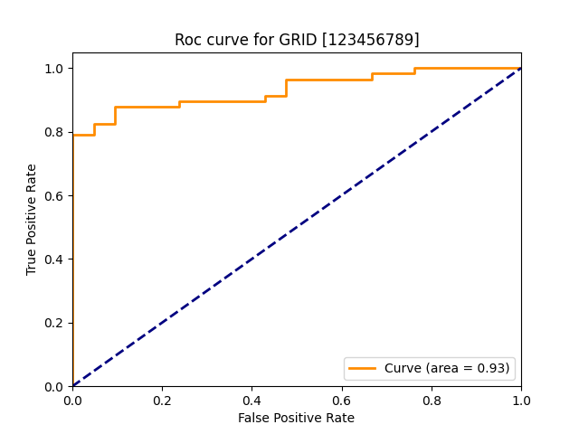 |
|
 |
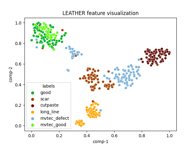
| leather | 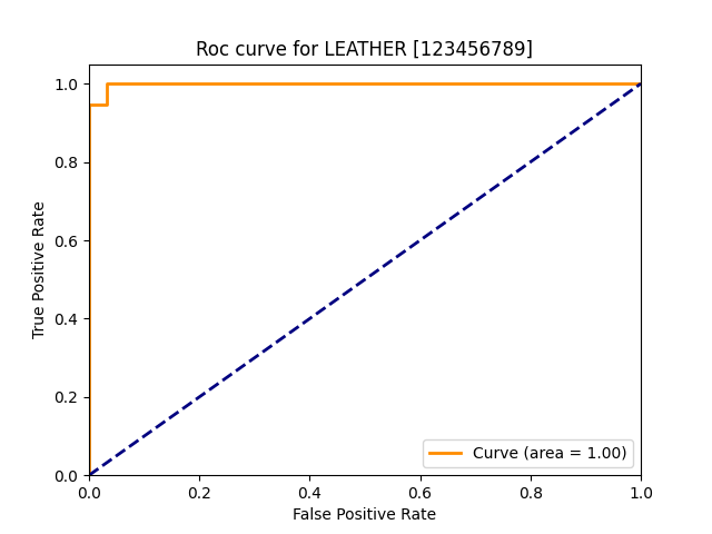 |
|
 |
| tile | 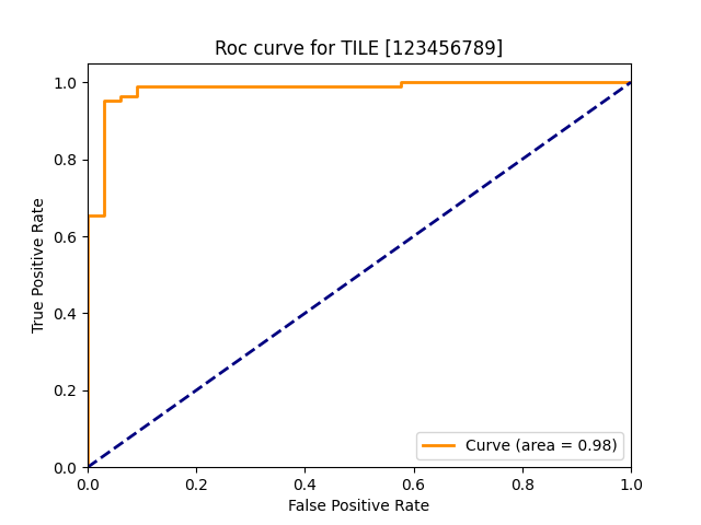 |
|
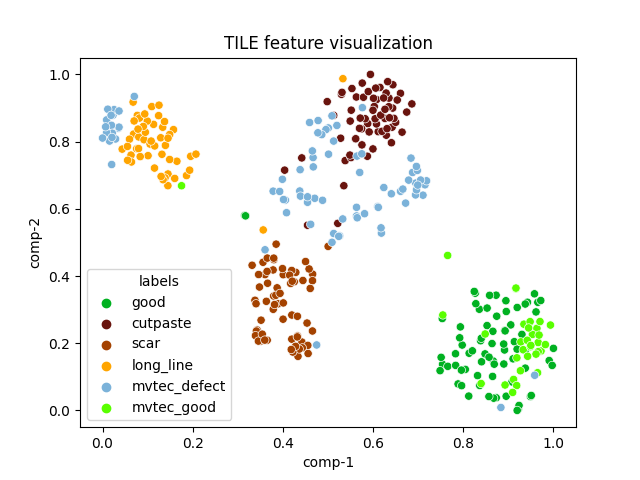 |
| wood | 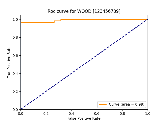 |
|
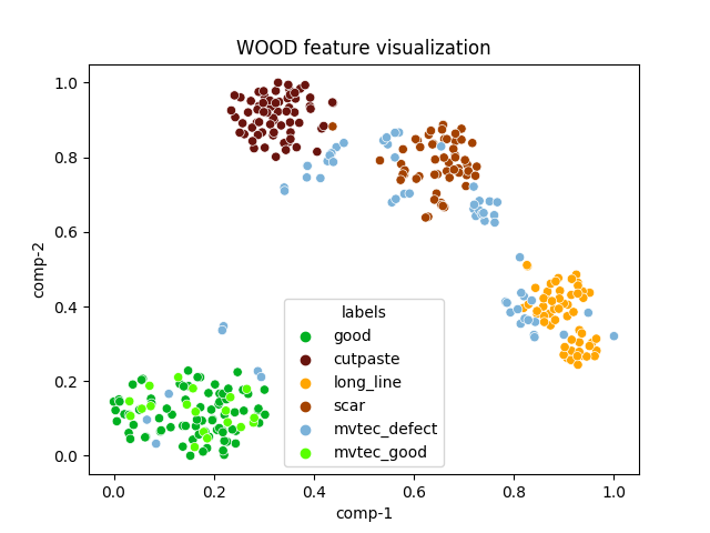 |