This small repository shows examples of visualizations of energy consumption patterns for commercial buildings. It uses data from the Open Energy Data Initiative (OEDI).
I present three visualization methods that can be used to display time series data with a high (sub-daily) sampling rate.
I have not seen this plot before, although I suspect I might not be the one to have this idea. This plot aims to show how the energy consumption profile of a group of buildings varies as a function of some characteristics. In the figure below, for example, I show how the day of the week affects the hourly energy consumption profile of primary schools.
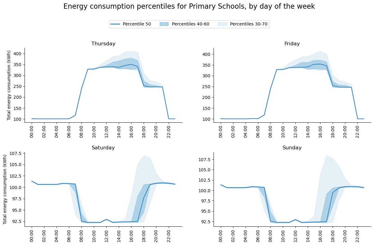
The dataset contains hourly energy readings for 365 days, but I want to show what a "typical" Thursday or Sunday looks like. At the same time, I want to show, to some extent, the spread around this typical value. I use the median reading (i.e., the 50th percentile) as the representative energy consumption value for each hour of the day. The median readings are plotted using a strong blue line. Then, I show other ranges of percentiles in increasingly pale colors. The range between percentiles 40 and 60 is in light blue, and readings even further out (up to the 30th percentile on the low end and the 70th on the high end) are in a paler shade of blue.
The quantile line plot hints at how values are distributed; at the same time, it keeps the chart clean and easy to use. Nevertheless, if we want to see the complete distribution of energy consumption profiles throughout the year, we can use what I termed a "ghost line plot". In this plot, each daily reading is displayed individually.
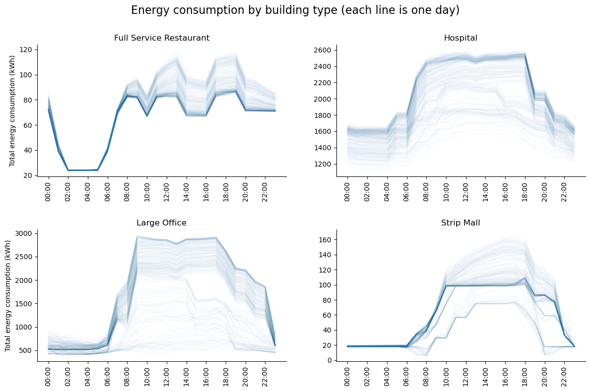
Each line is displayed at just 1% opacity to avoid cluttering the chart area. Overlapping lines increase the line weight in some areas and signal that many readings concur on the same or similar energy consumption values.
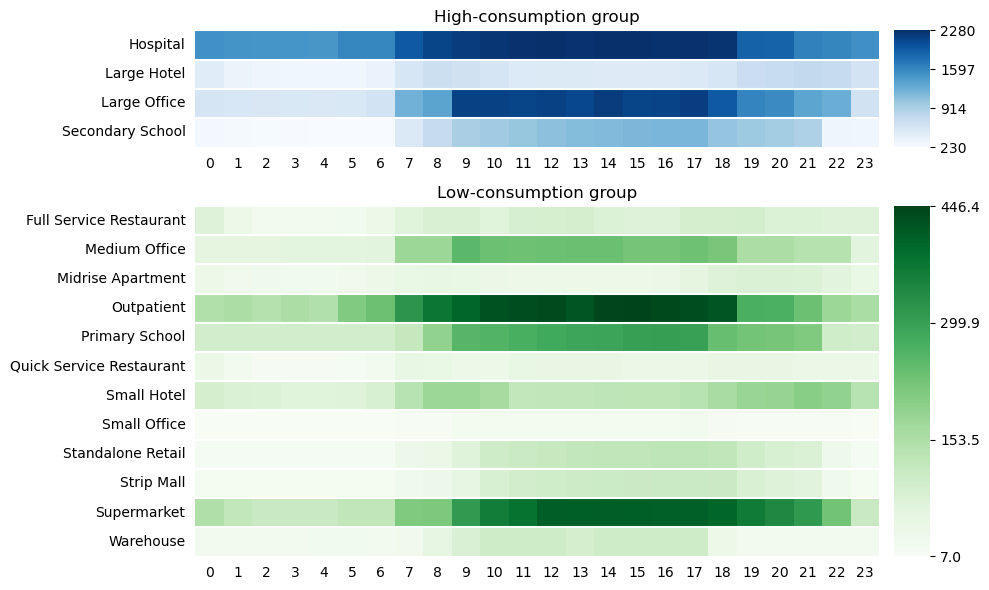
Heatmaps are a classic tool that uses color to succinctly convey information about where high and low values are to be found in the data. In the case of the energy consumption data, though, a few building types have a much larger hourly consumption than the others. Consequently, most building types would be represented by indistinguishable pale blue rectangles for most of the day, while a handful of buildings would have dark blue, at least during parts of the day. This is not ideal, as a heatmap is most useful when it uses a wide range of colors. Therefore, I decided to divide the buildings into high- and low-usage and present separate heatmaps (with different colors) for each.
Preparing the data was a long and not always straightforward process.
Dealing with time zones and daylight saving time was particularly challenging.
A data preparation script for the commercial buildings is available at preprocessing/preprocessing.py.
According to the OEDI documentation, each building is associated with the weather station whose readings have been used when creating the data.
A list of U.S. weather stations is available in energy/weather_stations_us.json.
The list is a filtered version of the one used in the meteosat/weather-station repository.
The filter script is at preprocessing/filter_weather_stations.py.
The final data is available in file preprocessing/commercial.csv.
The original OEDI data files are not provided because they take up several GBs.
Once downloaded from the OEDI website, they shall be placed in directory energy/commercial/.
All the code in the Python notebook and the Python scripts is released under the GPL v3.0 License.
See the LICENSE file in this repository.
The original OEDI dataset was released under the CC0 1.0 License. Weather station data was released under the CC Attribution 4.0 International Public License. This work has been inspired by a blog post by Gianluca Mauro.