Home
This repository contains documentation of code, datasets and models for the paper Obfuscation Revealed: Leveraging Electromagnetic Signals for Obfuscated Malware Classification published in ACSAC 2021.
Duy-Phuc Pham, Damien Marion, Matthieu Mastio, and Annelie Heuser. 2021. Obfuscation Revealed: Leveraging Electromagnetic Signals for Obfuscated Malware Classification. In Annual Computer Security Applications Conference (ACSAC). Association for Computing Machinery, New York, NY, USA, 706–719. DOI:https://doi.org/10.1145/3485832.3485894
The wiki structure is as follows
- The dataset for malware and benign executable (see Section 4 in the paper).
- Data acquisition code for reproducing the EM traces capture (see Section 5.2-6.1 in the paper).
- Pre-trained models contains all the pre-trained models for each scenario of ML and DL algorithms (see Section 6.2 in the paper).
- Analysis tools to reproduce the results of Machine Learning (ML) and Deep Learning (DL) models (Section 7 in the paper).
The dataset contains compiled ARM executables for both malware and benign dataset. Executables were compiled on Linux raspberrypi 4.19.57-v7+ ARM.
All executables can be executed directly on target device. The dataset was categorised in 5 different families: bashlite, gonnacry, mirai, rootkit, goodware. Except rootkits which require to be installed as follow:
Rootkit installation:
sudo insmod kisni-4.19.57-v7+.ko
For rootkit uninstallation:
sudo rmmod kisni-4.19.57-v7+.ko
Run it only once per target device reboot:
ARG1=".maK_it"
ARG2="33"
rm -f /dev/$ARG1 #Making sure it's cleared
echo "Creating virtual device /dev/$ARG1"
mknod /dev/$ARG1 c $ARG2 0
chmod 777 /dev/$ARG1
echo "Keys will be logged to virtual device."
For rootkit uninstallation:
echo "debug" > /dev/.maK_it ; echo "modReveal" > /dev/.maK_it; #Un-hide rookit
sudo rmmod maK_it4.19.57-v7+.ko; #Uninstall rootkit
For rootkit installation:
sudo insmod maK_it4.19.57-v7+.ko
For details of commands to execute malware on target device, please refer to subfolder cmdFiles
Note: This repository is made for research purpose. We are not liable or responsible for any damage caused by the installation of viruses or malware on your computer, software, equipment or other property due to your access to this repository or any other use of this repository.
The current repository contains all the scripts needed to interact with data acquisition interfaces published in the paper: "Obfuscation Revealed: Electromagnetic obfuscated malware classification".
This repository supports PicoScope® 6000 Series oscilloscope. To install required Python packages:
pip install -r requirements.txtWe use Raspberry Pi (1,2,3) in our setup. It is connected to the host analysis machine over Ethernet via SSH. The SSH IP configuration can be modified in generate_traces_pico.py .
ssh.connect('192.168.1.177', username='pi')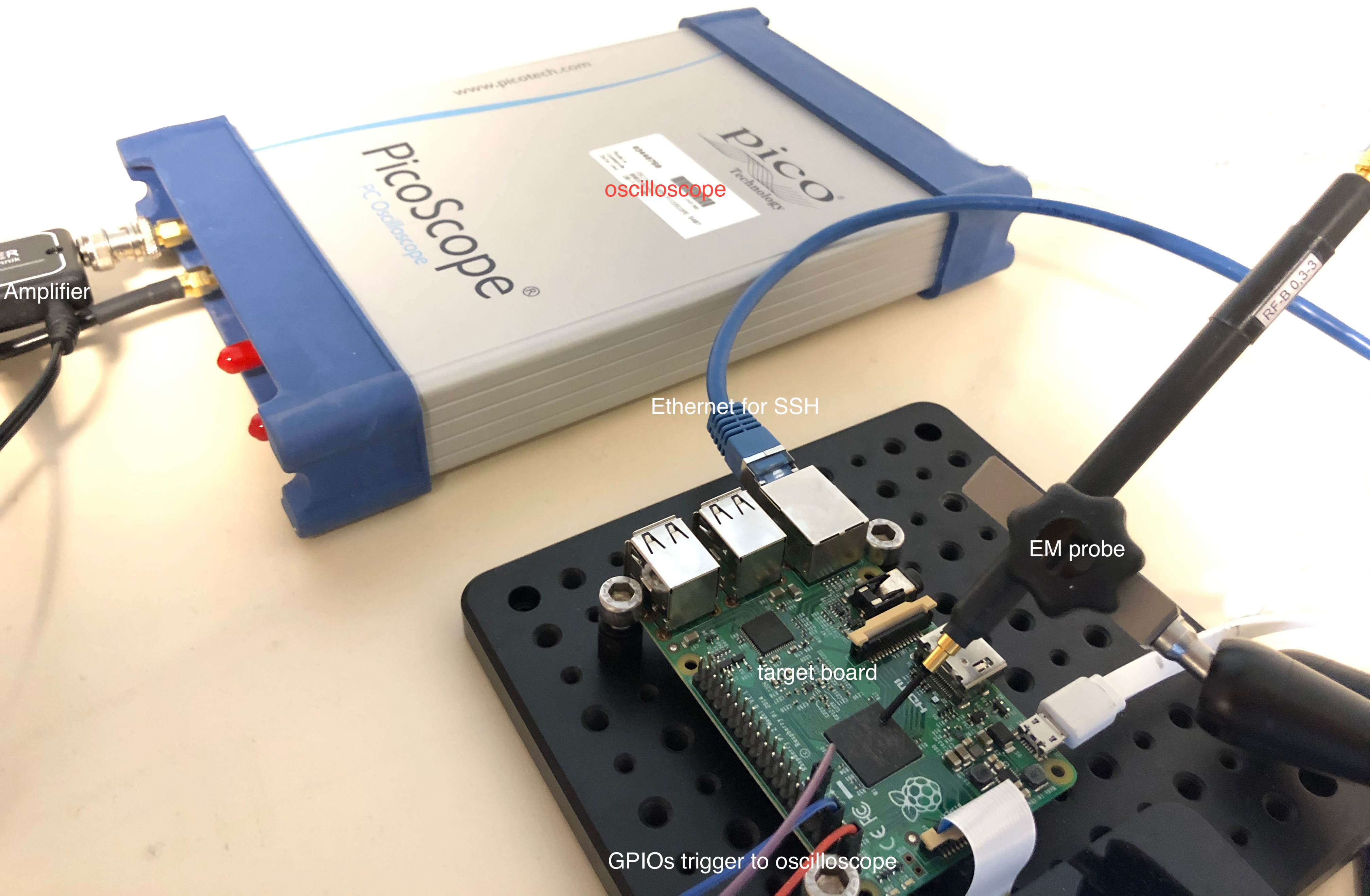
We use Langer PA-303 +30dB for amplifier, connected to a H-Field Probe (Langer RF-R 0.3-3) and Picoscope 6407 1GHz bandwith. The probe through amplifier is connected to port A, while the trigger from target device is connected to port B of the Picoscope.
To trigger the oscilloscope, we launch a wrapper program on the device. This wrapper will simply send the trigger and launch the program we want to monitor for the according time. It is automatically called by generate_traces_pico.py. You just need to precise its path on the monitored device. The compiled wrapper can be stored in /home/pi/wrapper or its path can be modified in generate_traces_pico.py . The wrapper has already configured Raspberry Pi Plug P1 pin 11, which is GPIO pin 17, as the trigger input for the oscilloscope.
You now need to provide the list of commands you want to monitor in a CSV-like file cmdFile.
The file must be of this form: pretrigger-command,command,tagEvery loop iteration will, for each line of the cmdFile, do the following:
- Execute the
pretrigger commandon the device via SSH - Arm the oscilloscope
- Trigger the oscilloscope and execute the monitored
command - Record the data in a file named
tag-$randomId.dat
Example of a command file for launching keysniffer:
sudo rmmod kisni,./keyemu/emu.sh A 10,keyemu
sudo insmod keysniffer/kisni-4.19.57-v7+.ko,./keyemu/emu.sh A 10,keyemu_kisni
Example of traces capture:
./generate_traces_pico.py ./cmdFiles/cmdFile_bashlite.csv -c 3000 -d ./bashlite-2.43s-2Mss/ -t B --timebase 80 -n 5000000This will capture 3000 traces from the oscilloscope, execute Bashlite malware on the target device with the path defined in cmdFile_bashlite.csv, and output traces to folder ./bashlite-2.43s-2Mss on host analysis machine. The oscilloscope will be executed in Block mode with sampling frequency "80". For more details please refer to data-acquisition repository.
This repository contains all the pre-trained models for each scenario and each Deep Learning (DL) and Machine Learning (ML) algorithms. Deep Learning models are compressed in 7z format, they need to be uncompressed before they can be used with other modules, use run_decompression.sh to decompress files.
To be able to run the analysis you (might) need python 3.6 and the required packages:
pip install -r requirements.txtTwo dataset are available to reproduce the results on the following website
https://zenodo.org/record/5414107
The two dataset are:
-
traces_selected_bandwidth.zip:the extracted bandwidth (40) of spectrograms from the testing dataset to reproduce the classification results presented in the paper, -
raw_data_reduced_dataset.zip:a reduce set of the raw electromagnetic traces to reproduce the end-to-end process (pre-processing and classification).
- Initialization
In order to update the location of the data, you previously dowloaded, inside
the lists you need to run the script update_lists.sh:
./update_lists [directory where the lists are stored] [directory where the (downloaded) traces are stored]
This must be applyed to directoies list_selected_bandwidth and list_reduced_dataset
respectively associated to the datasets: traces_selected_bandwidth.zip and raw_data_reduced_dataset.zip
For example:
./update_lists ./lists_selected_bandwidth/ ./traces_selected_bandwidth
- Evaluation of Machine Learning (ML)
To run the computation of the all the machine learning experiments, you can use
the scripts run_ml_on_reduced_dataset.sh and run_ml_on_extracted_bandwidth.sh:
./run_ml_on_extracted_bandwidth.sh [directory where the lists are stored] [directory where the models are stored] [directory where the accumulated data is stored (precomputed in pretrained_models/ACC) ]
The results are stored in the file ml_analysis/log-evaluation_selected_bandwidth.txt.
Models and accumulators are available in the repository named pretrained_models.
For example:
./run_ml_on_extracted_bandwidth.sh lists_selected_bandwidth/ ../pretrained_models/ ../pretrained_models/ACC
./run_ml_on_reduced_dataset.sh
The results are stored in the file ml_analysis/log-evaluation_reduced_dataset.txt.
- Evaluation of Deep Learning (DL)
To run the computation of all the deep learning experiments on the testing dataset with pre-trained models, you can use
the script run_dl_on_selected_bandwidth.sh:
./run_dl_on_selected_bandwidth.sh [directory where the lists are stored] [parent directory where the models are stored with subdirectories MLP/ and CNN/ (precomputed in pretrained_models/{CNN and MLP})] [directory where the accumulated data is stored (precomputed in pretrained_models/ACC) ]
The results are stored in the file evaluation_log_DL.txt.
For example:
./run_dl_on_selected_bandwidth.sh ../lists_selected_bandwidth/ ../pretrained_models/ ../pre-acc/
To train and store pre-trained models for the MLP and CNN architecture using the reduced dataset (downloaded from zenodo), you can use
the script run_dl_on_reduced_dataset.sh:
./run_dl_on_reduced_dataset.sh [directory where the lists are stored] [directory where the accumulated data is stored (precomputed in pretrained_models/ACC) ] [DL architecture {cnn or mlp}] [number of epochs (e.g. 100)] [batch size (e.g. 100)]
The models are stored as h5-files in the same directory with the name of the classification scenario.
Validation accuracies over all scenarios and bandwidths are stored in training_log_reduced_dataset_{mlp,cnn}.txt.
| scenario | # | MLP AC [ |
CNN AC [ |
LDA + NB AC [ |
LDA + NB AC [ |
| Type | 4 | 99.75% [28] | 99.82% [28] | 97.97% [22] | 98.07% [22] |
| Family | 2 | 98.57% [28] | 99.61% [28] | 97.19% [28] | 97.27% [28] |
| Virtualization | 2 | 95.60% [20] | 95.83% [24] | 91.29% [6] | 91.25% [6] |
| Packer | 2 | 93.39% [28] | 94.96% [20] | 83.62% [16] | 83.58% [16] |
| Obfuscation | 7 | 73.79% [28] | 82.70% [24] | 64.29% [10] | 64.47% [10] |
| Executable | 35 | 73.56% [24] | 82.28% [24] | 70.92% [28] | 71.84% [28] |
| Novelty (familly) | 5 | 88.41% [16] | 98.85% [24] | 98.25% [6] | 98.61% [10] |
- Using EM Waves to Detect Malware. Schneier on security. January 15, schneier. (n.d.). Retrieved January 21, 2022, from https://www.schneier.com/blog/archives/2022/01/using-em-waves-to-detect-malware.html
- ‘Skadlig kod kan upptäckas med elektromagnetiska vågor’. Computer Sweden. Accessed 21 January 2022. https://computersweden.idg.se/2.2683/1.761341/skadlig-kod-kan-upptackas-med-elektromagnetiska-vagor.
- ‘Identifying Malware By Sniffing Its EM Signature’. Tom Nardi. Hackaday (blog), 19 January 2022. https://hackaday.com/2022/01/19/identifying-malware-by-sniffing-its-em-signature/.
- Tracy, P. (2022, January 12). Raspberry pi can detect malware by scanning for electromagnetic waves. Gizmodo. Retrieved January 21, 2022, from https://gizmodo.com/raspberry-pi-can-detect-malware-by-scanning-for-electro-1848339130
- 新知答主. (n.d.). 探测电磁波就能揪出恶意软件,网友:搁这给电脑把脉呢?. zhuanlan. Retrieved January 21, 2022, from https://zhuanlan.zhihu.com/p/457343853
- Detecting evasive malware on IOT devices using electromagnetic emanations. The Hacker News. (2022, January 6). Retrieved January 11, 2022, from https://thehackernews.com/2022/01/detecting-evasive-malware-on-iot.html
- Matthew is PCMag's UK-based editor and news reporter. Prior to joining the team. (2022, January 10). No software required: Raspberry Pi uses electromagnetic waves to detect malware. PCMag UK. Retrieved January 11, 2022, from https://uk.pcmag.com/malware-protection-removal/138056/no-software-required-raspberry-pi-uses-electromagnetic-waves-to-detect-malware
- (2022, January 11). Raspberry pi peut désormais Détecter Les malwares sans logiciel. hitechglitz.com. Retrieved January 11, 2022, from https://hitechglitz.com/france/raspberry-pi-peut-desormais-detecter-les-malwares-sans-logiciel/
- Hill, A. (2022, January 9). Raspberry pi detects malware using electromagnetic waves. Tom's Hardware. Retrieved January 11, 2022, from https://www.tomshardware.com/news/raspberry-pi-detects-malware-with-em-waves
- (2022, January 11). Raspberry pi peut désormais détecter Les Logiciels malveillants sans Aucun Logiciel. Lesnumerics.com - Croire a la tecnologie. Retrieved January 11, 2022, from https://lesnumerics.com/raspberry-pi-peut-desormais-detecter-les-logiciels-malveillants-sans-aucun-logiciel
- Nihel Béranger (2022, January 11). Raspberry Pi Peut Détecter des virus Grâce aux Ondes électromagnétiques. Confluence News. Retrieved January 11, 2022, from https://confluencenews.fr/raspberry-pi-peut-detecter-des-virus-grace-aux-ondes-electromagnetiques/
- Spadafora, A. (2022, January 11). Raspberry pi can now detect malware without any software. TechRadar. Retrieved January 11, 2022, from https://www.techradar.com/news/raspberry-pi-can-now-detect-malware-without-any-software
- Gabriel. (2022, January 10). Un appareil basé sur raspberry pi utilise des ondes électromagnétiques pour détecter Les Logiciels malveillants. NetCost & Security. Retrieved January 11, 2022, from https://www.netcost-security.fr/actualites/69241/un-appareil-base-sur-raspberry-pi-utilise-des-ondes-electromagnetiques-pour-detecter-les-logiciels-malveillants/
- Singh, J. (2022, January 11). Raspberry pi can now be used to detect malware using electromagnetic waves. NDTV Gadgets 360. Retrieved January 11, 2022, from https://gadgets.ndtv.com/laptops/news/raspberry-pi-malware-detection-system-electromagnetic-waves-irisa-researchers-2701646