Affordable 9 DoF Sensor Fusion
For the individual maker, the last few years have seen a revolution in inertial motion sensing technology (Inertial Motion Units or IMUs) that consists of three components: the availability of inexpensive gyroscope/accelerometer/magnetometer sensors of high precision; the development of efficient and simple open-source 6- and 9-degrees-of-freedom (9 DoF) sensor fusion algorithms; and the availability of small, fast, and inexpensive microcontrollers. The combination of these three elements allows the creation of devices that can track absolute orientation with respect to a fixed Earth frame of reference with high accuracy in a very small package and for less than twenty dollars. My intention here is to explore this new world, demonstrate the kind of performance one can easily achieve, and illustrate some of the limitations too. I will start with the MPU-6050.

GY-521 Breakout Board with the MPU-6050 showing the Invensense MPU-6050 front and center (made in March (11th week of) 2012), the KB33 voltage regulator, and 2200 Ohm pull-up resistors on the SDA and SDL lines, which are broken out along with power and ground pins, auxiliary I2C lines, an address pin, and an interrupt pin.
The MPU-6050 is made by Invensense and consists of a MEMS (microelectromechanical system) accelerometer and gyroscope with 16-bit analog-to-digital converters for 60 micro g and 0.01 degree/second precision, respectively. The device was first released at the end of 2010 but is still state-of-the-art being used in the MPU-9150 device with an embedded magnetometer, which I will discuss later. The MPU6050 has been recently redesigned to become the MPU6500 gyro/accelerometer, shrunk 40% in size, and is being used in the newest MPU9250 9-axis sensor (more below). The MPU-6050 is available in many varieties of breakout board, which can be purchased for as little as $2 each, but is usually found on Amazon.com for ~$5. An astounding bargain considering the chip itself costs more than $5 in quantities of 100.
The MPU-6050 has a remarkable innovation called the Digital Motion Processor (DMP) integrated into the chip whose programming is proprietary to Invensense. It allows 6-axis sensor fusion calculations to be performed by the DMP at a fixed rate of 200 Hz and the results delivered to the host microcontroller in the form of a quaternion, Yaw, Pitch, and Roll, tap interrupts, portrait/landscape detection, etc. This capability is of major importance for the primary application of this chip in the smart phone and tablet markets. For the individual maker, as I will show, the use of the DMP is neither desirable nor necessary to get all the same functionality in a completely transparent fashion. I will discuss how to do this with open-source sensor fusion algorithms shortly.
The last of the three elements in our revolution is the microcontroller itself. I have chosen to work primarily with the 3.3 V 8 MHz Pro Mini Atmega 328P AVR microcontroller since it is small (2 cm x 5 cm), light (2 g), and cheap ($9 each when purchased by the dozen). I will also use the Arduino Uno which operates at 5 V and 16 MHz, and the Teensy 3.1. The latter is the epitome of affordable, powerful ARM microcontrollers being of the same size as the Pro Mini, about twice the cost (still cheap), and operating both at 3.3 V and up to 96 MHz processor speed with overclocking. This is overkill for the comparatively easy task of 9 DoF sensor fusion, as we shall see.
Hook up of the MPU-6050 to the Pro Mini is straightforward, only requiring connection of 3.3 V and ground and the SDA and SCL I2C lines (Pro Mini pins A4 and A5, respectively). There are pull-up resistors on most breakout boards so external ones are usually not required. Some breakout boards even have their own voltage regulator and can handle 5 V power. But the sensor is not 5 V tolerant and it is best to use a logic converter if you are using an Arduino Uno. There are several basic Arduino sketches that can be used to obtain scaled accelerometer and gyro data from the MPU-6050; I will be using and referring to this sketch.
Before we do anything else, let's get ourselves oriented. Think of a jet in the sky.

Gravity is down (+z axis). The Yaw is the angle (psi in the diagram) in the horizontal plane between the fuselage and true North (x-axis), the pitch (theta in the diagram) is the angle the nose makes with respect to the horizontal (x-y) plane, and the roll is the angle (phi in the diagram) of the wings about the long axis of the jet.

Figure 1
I'll get into more detail of what a typical sensor fusion sketch does in a bit; for now let's just take a look at some results to illustrate what the MPU-6050 can and cannot do. Here is plotted the Yaw, Pitch, and Roll output from a 6 DoF open-source sensor fusion algorithm using the MPU-6050 accelerometer and gyro data as input. We can see that the filtered Roll and Pitch are essentially zero for the sensor laying flat on the table and remain so for several minutes. The Yaw is slowly changing (about 1.8 degrees per minute here) due to gyro drift. Despite the drift, the Yaw returns to trend after slight rotations at the ~two minute mark. With only one axis as a frame of reference (gravity), we can specify two reference vectors (one parallel and one perpendicular) relative to the reference direction. That leaves one direction, the Yaw, undetermined. Due to the natural drift of any mechanical gyro, the Yaw will drift unless corrected by a second reference frame standard, like Magnetic North.

Figure 2
The proprietary sensor fusion algorithms in the MPU-6050 DMP do a better job than the simple open-source algorithm as shown here. Again, the Roll and Pitch are unchanging since there are two good reference axes. The Yaw is drifting although at a slower rate (~0.4 degrees per minute) than with the simpler sensor fusion filter. This device also responds quickly to changes in Yaw as seen at the ~one minute mark, returning to the previous Yaw drift trajectory after the excursion. We don't know what is in the proprietary sensor fusion filter used by Invensense but it is doing pretty well. Kudos to Invensense! We can guess that there is a sensor fusion filter, similar to what is in the sketch above, as well as low- and high-pass filters to smooth the output. In fact, we can get a sense of this by noticing the ~ten seconds it takes to get to a stable value of the Yaw, which then drifts at a slow rate. However, there is still drift which makes using this device, even with the improved algorithms in the DMP, as a reference for absolute orientation problematic. For smartphone and tablet orientation, the DMP is programmed to calibrate the acceleration and gyro biases whenever motion stops, so it will keep relative orientation accuracy over short times. But we can do much better than even the multi-talented DMP just by adding one other sensor device to provide a second orthogonal reference vector; the magnetometer.

Figure 3
Magnetometers are typically Hall-effect sensors that offer three-axis magnetic field measurement with high-precision and accuracy, for example, the HMC5883L by Honeywell achieves +/- 2 milliGauss resolution for a full-range of +/- 8 Gauss. These devices come in relatively inexpensive breakout boards, communicate via I2C, and can be easily added to the MPU-6050 to achieve very accurate, absolute orientation as shown here. With the addition of the Magnetic North reference vector to the system, we have three constraints that uniquely determine the orientation of our three axes and it shows: the Yaw, Pitch, and Roll are stable over many minutes within better than one degree precision and, depending on the care in the sensor calibration, as good as a few degrees absolute accuracy. Moreover, the Yaw now represents an absolute measurement; the edge of my desk that I use to align the sensor in all of these examples is about 45 degrees from true North. The power of 9 DoF sensor fusion is that it gives accurate, reproducible absolute orientation that 6 DoF sensor fusion cannot. So let's talk about sensor fusion.
Sensor fusion is a fancy name for error correction and at the highest level works like this. We form an estimate of the orientation which is usually represented by a Quaternion, which is a four-component vector that contains all the information needed to specify a unique direction in x/y/z space. The gyro output W in radians per second can be thought of as rates of change of this Quaternion:
dQ/dt = 1/2W x Q or Qt = Qt-1 x (1 + 1/2Wdt)
for each of the three spatial axes. Think of Q as our estimate of the sensor orientation. This just says that the rate of change of the Quaternion is half the gyro rate for each axis. Or, in terms useful for numerical integration, the new Quaternion estimate is equal to the old one times a function of the sensor rotation in a small time interval.
The error correction comes in by comparing the Quaternion estimate of the acceleration to that measured by the accelerometer:
Qt = Qt-1 x (1 + 1/2Wdt) + (AQ - Ameas) x beta x dt.
The estimate of Qt can be iterated to minimize this error term with the adjustable parameter beta controlling the rate of convergence to a stable answer. In practice, reasonable convergence can be achieved in two or three iterations meaning that we would like this error correction or sensor fusion filter to operate at a rate two or three times the output data rate of the sensor. For gyro and accelerometer output rates of 200 Hz, this means we want filter update rates approaching 1 kHz. In order to make use of our Quaternion estimate of orientation it is conventional to transform the four-component vector into a 3 x 3 rotation matrix, or into even simpler Yaw, Pitch, and Roll rotation angles. The best format will be dictated by the ultimate application of the sensor output. We will use the standard Attitude Heading Reference System (AHRS) reference frame applicable to aerial navigation, but there are other reference frames that might be more appropriate.
Note the simple error correction term gets us stable Roll and Pitch values but this orientation estimate will be subject to Yaw drift no matter how fancy the filter is since it lacks a second orthogonal reference vector to constrain the Yaw. With the addition of a magnetometer we can modify our orientation estimate by augmenting the error correction by comparing the Quaternion estimate of magnetic field with that measured by the magnetometer:
Qt = Qt-1 x (1 + 1/2Wdt) + [(AQ - Ameas) + (MQ - Mmeas)] x beta x dt.
Now we have an estimate that quickly converges to a unique solution that represents the absolute sensor orientation with respect to a fixed Earth reference frame. The Yaw, Pitch, and Roll values will always return to the same values no matter what the intervening motion when the sensor is reoriented back to a given direction.
All 9 DoF sensor fusion filters follow this basic approach but differ in the methods used to either construct the error terms, minimize the error terms, or both. See here for an excellent summary of methods and sources. The most common approach, yet also one of the more complicated ones, is the Kalman Filter (see here and here). Although these filters can be highly accurate, they require several matrix inversions and other matrix operations that are relatively expensive for small microcontrollers to handle quickly. Here is a nice discussion of sensor fusion using an easier-to-implement direction-cosine matrix approach that also requires matrix operations. In 2008, Robert Mahony developed a non-linear complementary filter to correct for gyroscope drift by using the gravity vector as a reference similar to the principle discussed above. In 2010 Sebastian Madgwick developed simple 6 DoF IMU and 9 DoF MARG (Magnetic, Angular Rate, Gravity) sensor fusion algorithms optimized for high filter update rates on small microcontrollers. Madgwick's paper is accessible and very well-worth reading. In addition to being fast, efficient, and accurate, the best thing about these filters is that they are open source! They are capable of matching the performance of the proprietary filters in the Invensense DMP in terms of accuracy and filter update rates, and allow full 9 DoF sensor fusion that the DMP cannot do as of yet.
I have implemented the open source sensor fusion algorithms for a variety of MARG sensors and have measured their performance using three microcontroller platforms for the sensor fusion filtering: the 3.3 V 8 MHz pro Mini, the 5 V 16 MHz Arduino Uno, and the 3.3 V 24/48/96 MHz Teensy 3.1. The sensor architectures, output data rates, and costs are compared in Table 1 and the performance characteristics of the filters are shown in Table 2.
 [Table 1]
These six different motion sensor solutions vary in their attributes, advantages, and limitations. Listed are typical sample rates and corresponding bandwidths in Hz. Also listed are typical costs and where to find breakout boards for your own testing. Of course, you can always make your own.
[Table 1]
These six different motion sensor solutions vary in their attributes, advantages, and limitations. Listed are typical sample rates and corresponding bandwidths in Hz. Also listed are typical costs and where to find breakout boards for your own testing. Of course, you can always make your own.
We have covered the MPU-6050 whose main limitation is the lack of a magnetometer. This can be remedied by adding a separate magnetometer, such as the Honeywell HMC5883L but with the disadvantage of increased complexity for the user (2 devices rather than one) and the problem of alignment between the two distinct devices. This is more of an issue in applications where high precision is required. For quadcopters, this solution will suffice. The GY-80 is in this category of multiple separate devices. It is the only 10 DoF sensor in the group having a BMP-180 pressure sensor integrated on the breakout board. The GY-80 class of multiple individual sensors on a board was state-of-the-art perhaps five years ago when multiple devices integrated into the same small package were unavailable. One can still find many examples of the GY-80-style multi-sensor board for sale at still rather elevated prices; some approaching $100. The GY-80 is a relatively inexpensive Chinese-made version of this solution with four individual sensors (six if you include the temperature sensors embedded in the BMP-180 and the L3G4200D gyro). The complexity for the user has been diminished somewhat by the on-board integration and some care has been taken to get the relative orientation of the devices correct. Still, one can do better.
The modern approach is to integrate multiple sensors into one small package. Popular examples of this are the MPU-9150 from Invensense and the LSM9DS0 from ST Microelectronics, both of which combine an accelerometer/gyro with a Hall-sensor magnetometer into one 4 mm x 4 mm package. ST Microelectronics is a leader in MEMS gyro design and has the largest market share, although Invensense has the smallest 9-axis solution and is in a position to challenge that lead.
The MPU-9150 uses the MPU-6050 accelerometer/gyro discussed above married with an Asahi Kasei AK8975A magnetometer. The AK8975A magnetometer is limited to one-shot data output so a register write to the device must be made each time magnetometer data is desired. The resolution of the magnetometer is +/- 3 milliGauss with a full-scale range of +/- 12 Gauss. The DMP still does 6 DoF sensor fusion but there is no way to get magnetometer data into or out of the DMP to get true 9 DoF; Invensense announced a 9 DoF sensor fusion solution for multiple microcontroller platforms at their latest (June 11-12) Developer's Conference. For the individual maker, microcontroller-based sensor fusion will have to do for now. There is a comprehensive library for the MPU-6050 and MPU-9150 developed by Jeff Rowberg et al. at I2CDevLib; most folks find it a bit hard to use but it does have a 'hack' on the DMP usage which works well. I created a more transparent C++ Arduino sketch that accesses the data from all the MPU-9150 sensors and does 9 DoF sensor fusion on the results using Madgwick's and Mahony's sensor fusion filters. You can find that sketch here.
The LSM9DS0 offers similar capability as the MPU-9150 without the DMP. I find the LSM9DS0 data sheet a bit easier to negotiate than the MPU-9150 data sheet and Jim Lindblom of Sparkfun has created an excellent library for this device, which includes a sensor fusion capability I added using the same open-source sensor fusion algorithms as those discussed above. The magnetometer in the LSM9DS0 offers several output data rates from 3 to 100 Hz and excellent resolution at +/-80 microGauss with a full-scale range up to +/-12 Gauss. In future versions of this integrated sensor solution ST Microelectronics will be adding an embedded processor, like Invensense's DMP, for off-loading the sensor fusion function from the host microcontroller, and integrating additional devices such as a pressure sensor into smaller and smaller packages. Freescale is also active in the highly-integrated motion sensor market and hopes to compete with the MPU-9150 and LSM9DS0 with its new offerings (see here and here). More sensors integrated into smaller packages is the current trend in motion sensing and I expect tremendous near-term progress by these three leaders toward increasing capability, and decreasing footprint and cost driven by the smart device market. What a wonderful trend for the individual maker!
The epitome of small-scale sensor integration is represented by the MPU-9250 by Invensense. It marries the MPU-6500 accelerometer/gyro, which allows either SPI or fast I2C communication with a host, with the AK8963 magnetometer, which allows continuous data output at either 8 or 100 Hz rates and +/-1.5 milliGauss resolution with full-scale range of +/- 48 Gauss, all in a small 3 mm x 3 mm package.
A teardown comparison between the LSM9DS0, MPU9250 and BMX-055 9-axis motion sensor solutions is discussed here. I haven't mentioned the BMX-055 by Bosch since I just discovered it and am in the process of making my first breakout boards and writing a sensor fusion code for it. I'll have more to say about its performance later. For now, let me quote liberally from the above teardown review...
"The three components use different packaging, with footprints that range from 4x4 mm (16 mm²) for the STMicroelectronics part to 3x3 mm (9 mm²) for the InvenSense device. STMicroelectronics and Bosch Sensortec use LGA packages, while InvenSense uses a QFN package.
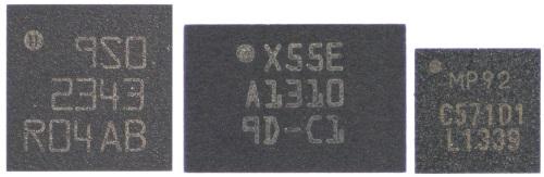
ST Microelectronics LSM9DS0, Bosch's BMX-055, and Invensense's MPU9250 9-axis motion sensors.
"Strong differences in internal structure emerged after we removed the epoxy resin. For example, STMicroelectronics and Bosch use five die, but InvenSense only uses two -- one die for a six-axis accelerometer/gyroscope and one for a three-axis magnetometer."
"Thus, each player varied widely in the silicon area they used, from 19 mm² for STMicroelectronics to 14 mm² for Bosch and just 8 mm² for InvenSense. More silicon die requires more wire bonding for connecting them. The STMicroelectronics IMU uses 76 wire bondings, compared to 25 for the InvenSense device."
"STMicroelectronics uses a single MEMS die for the six-axis accelerometer/gyroscope, shrinking the size of the six-axis function by more than 30% over its previous combo solution, which used two dice."
"The Bosch component is the only nine-axis MEMS IMU with all its functions (accelerometer, gyroscope, and magnetometer) developed and manufactured by the same player. The BMX055 integrates the second generation of Bosch's geomagnetic sensor with the three-axis support in a single die compared to three separates die for the previous generation."
"InvenSense's latest nine-axis IMU integrates a new three-axis gyroscope, now using a single vibrating structure, versus three different structures for the previous generation. This new design results in 40% shrinkage in the three-axis gyro area."
"A second benefit of this new design is that its Nasiri process has been changed. Cavities which were traditionally etched in the ASIC to allow MEMS structures to move are no longer used, resulting in a cost reduction."
"The device also integrates a new three-axis magnetometer, which features an almost 40% size reduction from the previous generation."
You can buy(!) the entire report here.
Let's talk about performance. One of the most important performance figures of merit is the sensor fusion filter rate. This determines how quickly the iteration to a stable quaternion is achieved and, as you might imagine, depends more on processor speed and the sensor fusion algorithm than the details of the motion sensor.
 [Table 2]
Typical sensor fusion rates for the six motion sensor solutions examined here on four microcontroller platforms. The filter update rates depend on the processor speed and top out at a rate limited by the sampling rate and averaging methods chosen.
[Table 2]
Typical sensor fusion rates for the six motion sensor solutions examined here on four microcontroller platforms. The filter update rates depend on the processor speed and top out at a rate limited by the sampling rate and averaging methods chosen.
The table is evolving; I fixed the compiler error I was having on the Teensy 3.1 by installing an updated Adafruit graphics library, so now I have complete Teensy data up to 96 MHz clock speed. Also, I discovered (thanks Paul Stoffregen) I was not using the 400 kHz i2c rate on Teensy as I thought; this has now been sorted out. I also had to implement a filter update rate averaging scheme which brought many of the previously reported instantaneous rate down about ten percent. When the filter update rates are greater than the sample output rate, the microcontroller has to wait for the sample output and this can cause a variety of instantaneous filter update rates to be reported, making performance comparisons between microcontrollers difficult without some kind of rate averaging. Now all these data are reported on more or less the same footing, which allows a straightforward comparison between the different microcontroller platforms and sensor solutions. Let's dig into the data.
The first observation is that the filter update rates for the MPU-6050 accelerometer/gyroscope are faster than those of most of the other sensors with any given microcontroller. This is because there are only two sensors to read, and both are faster than the magnetometers in the other sensors. The exception is the LSM9DS0, of which we shall say much more. Another consequence of the absence of a magnetometer is the filter itself has fewer operations and is, therefore, usually faster to run.
We can see that the filter update rates are roughly proportional to the processor speed, which is expected. Even the 8 MHz Pro Mini is capable of reaching filter update rates well above 100 Hz and, with the Mahony filter, is keeping up with the sensor sample output rates. The Uno at 16 MHz is getting into the ideal filter update rate regime with update rates approaching twice the data sampling rates. The Teensy can update the sensor fusion filter at a much faster rate (>1000 Hz) than necessary in most cases. The dependence on processor speed can be better seen in the following plot:

The filter update rate average smooths out the rate jitter I was seeing before but introduces some additional overhead that diminishes the reported rate; for the Pro Mini the rate is 10% less with the averaging than the case when only the instantaneous rate is reported. This is mostly due to certain processor tasks such as updating the display, etc. that interrupt the smooth flow of the sensor fusion; the rate is further diminished by 10% when I turn on the Serial Debug output. In other words, and no surprise, overhead matters. For maximum efficiency the microcontroller should be asked to do only those tasks necessary to achieve the application goal. The rates depend also on various code efficiencies being achieved, for example, the temperature doesn't have to be read at the same rate as the accelerometer and gyro. So while the averaging allows some sensible comparison between the processors, the points in the plot should be thought of as having +/-10% error bars. The plot shows that the sensor fusion filter update rates rise approximately linearly with processor speed, as one should expect. The 32-bit ARM processors significantly outperform the 8-bit AVR processors. But there is something more going on here.
Why does the LSM9DS0 allow significantly higher sensor fusion filter update rates, especially at the fastest processor speeds where the difference between the LSM9DS0 filter update rate and that of the nearest rival is more than 30%? The sketches are not exactly the same and I investigated whether using interrupts to prompt data acquisition, like used in the LSM9DS0 sketch, was making the difference compared to the STATUS register polling I was using elsewhere. The short anwer is no; there was a slight (maybe 5%) change with the interrupt approach, but none of the other sensors or platforms could approach the LSM9DS0 filter update rates at the high end. For those sensors solutions that depend on multiple separate devices, communication across the I2C bus even at the 400 kHz I am using could limit the effective sample read rate and thereby reduce the overall filter update rate. It is also curious that the GY-80 and MPU-6050 + HMC5883 sensor solutions behave so similarly slowly. I suspect the common HMC5883 magnetometer to be the culprit. Can we verify this hypothesis by comparing the details of the two magnetometers: the HMC5883 and the LIS3MDL? No, the specs seems pretty similar.
At the highest processor speeds, the update rates are far higher than the data sample output rates, so the processor has a lot of time while it is waiting for new data to iterate through the sensor fusion filter. The filter itself should be the rate limiting step and, as far as I can tell, the filters are 'identical', so the rates should be also. I am missing something here, and I still suspect that the differences in filter update rates at the limit of high processor speed are related to the performance of the magnetometers but I don't yet know how.
As you can see, I have also started to experiment with using another ARM processor, the STM32F401 which runs at 84 MHz and has a single-precision floating point engine embedded in the core. It is performing even better with the MPU-6050 than the Teensy 3.1. I am working on getting timing data for the other sensors. It is a bit harder to program than the Teensy 3.1 using Teensyduino, the Arduino-like programming created and maintained by Paul Stoffregen at pjrc.com/Teensy but it is one of a family of inexpensive and very powerful ARM microcontrollers perfectly suited to sensor fusion and motion control.
Let's talk about accuracy and stability. Absolute orientation with respect to a fixed Earth reference frame is a solved problem. The simple open-source 9-axis sensor fusion algorithms achieve this goal but with what accuracy? Below is a plot of the performance of the MPU-9250 9-axis motion sensor running Madgwick's sensor fusion filter using the Teensy 3.1 operating at clock speed of 96 MHz, which achieves average sensor fusion filter update rates of 2000 Hz.

Figure 5 Yaw, pitch and roll from an MPU-9250 using Madgwick's sensor fusion algorithm running on a 96 MHz Teensy 3.1 at a filter update rate of 2000 Hz. Data was collected over a half-hour period.
The data are captured from the initialization of the device to the end of 1800 seconds of continuous run time where periodically I picked up the breadboard containing the controller and MPU-9250 and moved around the room and waved it about. The goal was to measure stability of the output over a reasonable use time and determine how reproducibly the device returned to its reference orientation when placed back at the edge of my desk. We can see that after each excursion, lasting anywhere from 10 seconds to nearly a minute, where I tried to simulate vigorous motion the device returned very rapidly to its reference orientation readings, which at the edge of my desk were 131 degrees yaw, and 0 degrees pitch and roll. The relative error of the static readings is less than one degree; the slight upward tilt of the yaw is likely due to imprecise placement of the device at the edge of my desk after the last excursion. My interpretation of this experiment is that the relative orientation achievable is a degree or less in each direction and is very stable to all kinds of intervening movement.
Absolute accuracy is harder to quantify. I mean I would like to know how far off the x-axis is from true North when I orient the device such that it reads 0,0,0 for yaw, pitch, and roll. This is going to depend on how well the accelerometer and gyro are calibrated (very well) and how well the magnetometer is calibrated (not so well). The latter is going to limit the absolute accuracy. Here is what I did: I taped a piece of paper to my dining table and drew a line that corresponds to true North according to my hiking compass after correcting for the local declination. Then I removed the compass so as to reduce stray magnetic fields and oriented the MPU-9250 sensor device such that the x-axis was aligned with true North as determined previously with the compass. The roll and pitch will remain at zero and the yaw registered by the sensor will give the absolute orientation error. I found this to be 4 +/- 3 for the MPU-9250 running in the above configuration powered by a LiPo battery.
This not too bad an average absolute deviation, but the jitter is somewhat disappointing. The accuracy of any magnetometer-based sensor fusion is going to strongly depend on the accuracy of the magnetometer calibration. Just calibrating by min/max averaging on the axes as we have done here might not be sufficient if the response surface is not spherical; and there is no reason to expect it to be. There are sophisticated methods for magnetometer calibration and, if absolute accuracy is your goal, you might have to investigate them.
For instance, one of the most challenging motion sensor applications is determination of relative position. Imagine you are at a large Mall; can the motion sensor tell you where you are relative to where you came in. Leave alone absolute position, which is extremely challenging, even relative position determination quickly goes awry when faced with +/- 3 degree variations in absolute orientation. How could we have this jitter when Figure 4 shows such stable performance. Well part of the answer is that my true North experiment took place with a laptop in the vicinity; when I removed the laptop the result changed a bit to 5 +/- 2 degrees. And this illustrates the problem. Even a properly calibrated magnetometer will be strongly influenced by environmental variations in magnetic field (called soft iron effects) that will quickly render even relative position calculations nearly useless without some sophisticated correction algorithms. Challenging? Yes, but fun too!
We have just scratched the surface in our discussion of accuracy, but just on the basis of the filter update rates and the stability achieved here, any of these MARG sensor solutions coupled with open-source 9 DoF sensor fusion algorithms run on your favorite microcontroller provide adequate performance for all but the most demanding motion sensing tasks. And all for a modest total cost of between $20 and $50 depending on (mostly) the choice of sensor and (to a lesser extent) microcontroller.