Spatial join benchmarks (from Scipy 2020 talk)

[jorisvandenbossche]

I have been benchmarking our current spatial join algorithm, based on the benchmarks from https://github.com/Quansight/scipy2020_spatial_algorithms_at_scale (Scipy 2020 talk showing benchmarks with spatialpandas, pdf slides of the presentation are included in the repo, and there is a link to the youtube video as well).
In my fork of that repo, I added some extra cases using dask-geopandas instead of spatialpandas, and did some additional experiments: https://github.com/jorisvandenbossche/scipy2020_spatial_algorithms_at_scale

Benchmark setup

The benchmark code downloads GPS data points from OpenStreetMap (2.9 billion points, but clipped to US -> 113 million points). The point dataset is spatially sorted (with Hilbert curve) and saved as a partitioned Parquet dataset.
Those points are joined to a zip codes polygon dataset (tl_2019_us_zcta510). For the benchmarks, different random subsets of increasing size are created for the polygon zip layer (1-10-100-1000-10000 polygons).

So basically we do a spatial join (point-in-polygon) of a Parquet-backed partitioned point dataset with a in-memory (single partition) polygon layer. The left points is always the same size (113M points), the right polygons GeoDataFrameis incrementally larger (this are the different rows in the tables below).

The results are from my laptop, using a distributed scheduler started with 1 process with 4 threads (and a limit of 8GB memory).

Initial run

I created an equivalent notebook of the benchmark but using dask-geopandas instead of spatialpandas: https://github.com/jorisvandenbossche/scipy2020_spatial_algorithms_at_scale/blob/master/02_compared_cases/dask_geopandas/spatially_sorted_geopandas.ipynb

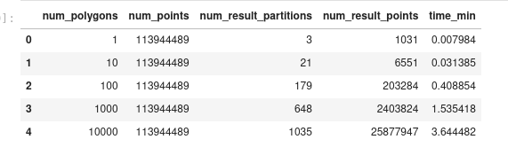
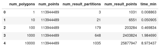
First, I also ran this with using a plain GeoPandas GeoDataFrame as the polygon layer. But then we don't make use of the spatial partitioning information (we just naively do a sjoin of each partition of the points dataset with the polygons geodataframe), because currently the dask_geopandas.sjoin will not calculate spatial partitioning information, but only make use of it if already available. So for those cases, the spatially sorting doesn't add much value, and the size of the polygon dataset doesn't matter much. And, spatialpandas does calculate the spatial partitioning information, so for an equivalent benchmark, I converted the polygon geopandas.GeoDataFrame into a dask_geopandas version (with 1 partition) and calculated the spatial partitioning. At that point you clearly see that for the small polygon dataset (only a few polygons), this helps a lot as we only need to read in / join a few of the point partitions.

For the smaller data, spatialpandas and dask-geopandas were doing very similarly, but for a larger polygon dataset (for a point-in-polygon join), geopandas started to be a lot slower.

Spatialpandas:

Dask-GeoPandas:

However, while looking into what the reason of this slowdown could be, I noticed that we were using the default predicate="intersects" of sjoin (that's the only predicate that spatialpandas supports). But for a point-in-polygon, I can explicitly pass predicate="within", and it seems that for the larger case, this makes it quite a bit faster:

Now it is actually very similar to the spatialpandas result.

(I was actually assuming I was doing an "within" join, and for that case, we switch left/right internally in the sjoin algo, so I was thinking that that might play a role, only to notice I wasn't actually doing a proper point-in-polygon sjoin (although of course for points/polygons "intersects" is essentially the same, but thus doesn't have the same performance characteristics)

Partitioning / spatially sorting the right polygon layer

Something I was thinking that could be a way to further improve the performance, was to also split and spatially shuffle the right (polygon) layer. I tried this for the largest case of 10,000 polygons, cut it in 10 partitions and shuffled it based on Hilbert distance. See https://nbviewer.jupyter.org/github/jorisvandenbossche/scipy2020_spatial_algorithms_at_scale/blob/master/02_compared_cases/dask_geopandas/spatially_sorted_geopandas.ipynb#Joining-with-a-partitioned-/-spatially-sorted-GeoDataFrame

However, this didn't actually improve much (in this case) ..

Some thoughts on why this could be the case:

• Note that the left (points) layer is already spatially sorted
• By splitting the polygons, each underlying geopandas.sjoin call is with fewer polygons and should be faster. But, we also slightly increase the number of sjoin calls (because the spatial partitions of left/right don't match exactly), creating more overhead. And the time spent in bulk_query is in the end also relatively limited, so it might be that the speed-up in the actual query isn't sufficient to overcome the added overhead.
• The final resulting number of matches the tree has to find is the same, so maybe it's quite efficient in short cutting when there is no overlap. Meaning, if you do a query with 1000 polygons that should give 1000 matches, or with 10_000 polygons that also gives 1000 matches, it's maybe not that much slower in the second case (wild guess here, didn't actually check this).

Note that the above was actually from running it on a subset of the point data, because with the full dataset I ran into memory issues.

Memory issues

While trying out the above case of using a partitioned dateset (with multiple partitions) for both left and right dataframe in the sjoin, I couldn't complete the largest benchmark on my laptop with the limit I set of 8GB memory for the process. Watching the dashboard, the memory usage increased steadily, at some point it started to spill data to disk (dask has a threshold for that (percentage of total available memory) that can be configured, default is already 50% I think), and things started to generally run slow (tasks took a long time to start), and a bit later I interrupted the computation.

From looking at the task stream, it seems that in this case it is loading too many of the point partitions into memory upfront, exploding memory. In "theory", it should only load 4 partitions in memory at a time, since there are there are 4 threads that then can do a spatial join with it. But while the computation is running, the number of in-memory "read-parquet" tasks continuously increases, and at 60 it starts to spill to disk and run slow, and at 90 I interrupted the process.

I ran it again to make a screencast. Now it only didn't start spilling to disk, but still showed the large increase in memory usage / many in-memory "read-parquet" tasks: https://www.dropbox.com/s/q1t2ly6x2f2gwb2/Peek%202021-09-17%2021-58.gif?dl=0 (a gif of 100MB is maybe not the best way to do this, an actual video file might be easier ;))

So when not having a single-partition right dataframe, there is something going on in executing the graph that is not fully optimal. I don't really understand why the scheduler decides to read that many parquet files already in-memory (much more than can be processed in the subsequent sjoin step with 4 threads).
Some observations:

• There is a lot of "unmanaged memory" according to dask. See also this blogpost about this topic: https://coiled.io/blog/tackling-unmanaged-memory-with-dask/ (and docs: https://distributed.dask.org/en/latest/worker.html#memory-not-released-back-to-the-os)
• It might be that dask doesn't really know how "big" the GeoDataFrames are. And for the geometry column, we indeed give a gross underestimation at the moment in geopandas (https://github.com/geopandas/geopandas/blob/9e0770b470d02b8db2887e6fd22076be03b934e4/geopandas/array.py#L1092-L1094, i.e. only the bytes of the pointers to the Python objects, so not even the size of the pygeos Python objects, let alone the memory of the actual coordinates in GEOS). We could maybe give a better estimate here, although estimating it eg on the number of coordinates is also costly to compute.
• ... (further to investigate)

Parallelization of the spatial join

While doing many tests trying to understand what was going on, I actually also noticed that when running it with the single-threaded scheduler (easier for debugging errors), it was not actually much slower ... In other words, running this spatial join benchmark with 4 threads in parallel didn't give much parallelization benefit.

Testing some different setups of the local cluster, it seemed that running this benchmark with 4 workers with each 1 thread was actually faster than with 1 worker with 4 threads (so basically using processes instead of threads).

While the STRtree query_bulk releases the GIL (and thus can benefit of multithreading), it seems that the sjoin in full doesn't release the GIL sufficiently to be efficient with multiple threads.

Profiling a single geopandas.sjoin call on one of the partitions gives the following snakeviz profile:

Interactive version: https://jorisvandenbossche.github.io/host/sjoin_snakeviz_profile_static2.html

So for this specific one (for each partition of the dataset it will of course give a somewhat different result), you can see that the actual bulk_query is only 19% of the time, calculating the bounds is another 10%, and the actual cython join-algo from pandas (get_join_indexers) is only 2 %. And AFAIK, those are the most relevant parts of this function that release the GIL.

Things we could look into to improve this:

• Improve the general basic geopandas.sjoin performance:
  • We could try to remove some python overhead: avoid unnecessary copy, (re)set_index, improve the performance of set_geometry, ..
  • Investigate if it is actually beneficial to calculate the total_bounds, instead of creating the tree and letting the tree see that there is nothing in common (reason: I noticed that the calculation of the total bounds actually take a considerable part of the sjoin, more than the actual bulk_query). Or, have an option to skip the check (which could be useful for dask-geopandas version in case we have spatial_partitioning information where we basically already did a total_bounds check)
• Release the GIL in the STRtree creation (now we only release it in the query_bulk)
• Work with larger partitions? (with the assumption that doing an sjoin on larger data increases the time in the actual query algo, and relatively reduces the python overhead)

The last item is something that I tried, creating a version of the partitioned Parquet point dataset with 100 partitions (each partition ~ 1 million points) instead of the original (from the upstream benchmarks) datasets with 1218 partitions (each partition ~100k points). Link to notebook
This didn't improve things for the smaller benchmark cases (because we needed to load larger partitions into memory, even when needing a small subset), but for the case with the largest polygons layer, it improved things slightly (3.1 min instead of 3.4min)

---

Summarizing notes

A too long post (I also spent too much time diving into this .. :)), but a few things we learnt:

• Never forget to check the predicate you are using (and experiment with it, as it can probably depend on your exact dataset)
• Dask-geopandas and dask-spatialpandas in the end perform more or less the same
• When your right dataframe is also partitioned, there still seems to be some memory issues that's worth investigating further
• Consider whether using more processes vs more threads in your cluster (it will also depend on the exact operations you are doing, but so for spatial join multithreading is not super ideal at the moment)
• There is room to improve the performance of the geopandas.sjoin

[brendan-ward]

@jorisvandenbossche thanks for exploring this and summarizing your findings here!

if it is actually beneficial to calculate the total_bounds, instead of creating the tree and letting the tree see that there is nothing in common

Internally, STRtree has to calculate the bounds of each geometry, and based on the tree algorithm derives bounds for the entire tree. This is checked early on in the query process. So it seems that the major tradeoff is between calculating bounds of all geometries to derive total_bounds up front to determine no overlap, or constructing the tree (internally based on bounds) then using query / query_bulk to check for overlap.

If there IS overlap and you need to query the tree (hopefully the most common case), then we're calculating bounds 2x (first for total_bounds, then again within tree), so that does seem potentially inefficient. If total_bounds are already known, then it seems worth it to check that in advance, but otherwise perhaps we should not do that by default?

Refs:

• ENH: check for non-overlapping bounding boxes in overlay and sjoin geopandas#1708
• ENH: Add bounds checks to sjoin, overlay (#1708) geopandas#1851

I don't know if the addition of the bounds check was benchmarked to determine if it is indeed faster.

[jorisvandenbossche]

@brendan-ward only seeing your response now. In the meantime I just did some benchmarks on the total_bounds / tree creation in case of no overlap, and opened geopandas/geopandas#2116 with that.

So it seems that the major tradeoff is between calculating bounds of all geometries to derive total_bounds up front to determine no overlap, or constructing the tree (internally based on bounds) then using query / query_bulk to check for overlap.

From that one case I benchmarked in the linked issue, constructing the tree is (as expected) still somewhat slower as calculating the total bounds (but also not by many orders of magnitude; in this case 3x, but should probably check with a larger dataset)

If there IS overlap and you need to query the tree (hopefully the most common case), then we're calculating bounds 2x

Indeed, and ideally we have a way to avoid that (even if we keep it by default in geopandas, we could still add a keyword to disable it (although it would be a very niche keyword ..), and have dask-geopandas disable it if it already checked the spatial_partitioning bounds beforehand.

If total_bounds are already known, then it seems worth it to check that in advance, but otherwise perhaps we should not do that by default?

In general, geopandas.sjoin doesn't know if the total_bounds are known (unless we would start caching such attributes on the GeometryArray, which might actually an interesting (different) topic to discuss). So either we somehow pass that information to sjoin (eg with the keyword to disable the total_bounds check that you can set if you already yourself checked it, as mentioned above), or either we simply remove the check. Not sure if there are other options?

[gjoseph92]

Hey @jorisvandenbossche, just stumbled across this.

it seems that in this case it is loading too many of the point partitions into memory upfront, exploding memory. In "theory", it should only load 4 partitions in memory at a time, since there are there are 4 threads that then can do a spatial join with it. But while the computation is running, the number of in-memory "read-parquet" tasks continuously increases, and at 60 it starts to spill to disk and run slow, and at 90 I interrupted the process

This sounds a lot to me like a longstanding problem with the scheduling algorithm called "root task overproduction". See dask/distributed#5555 and dask/distributed#5223 for more details. I'm concerned and a little surprised you got up to 90 root tasks in memory with just one worker, but not that surprised. The more that the scheduler is under load (dashboard, many tasks, etc.), and the faster the root tasks are, the more overproduction you'll see, since there's more latency between when a root task finishes and when the scheduler can send the worker a new thing to do.

There's not really a fix for this right now, unfortunately. The best thing you can do to alleviate it task fusion. For DataFrames, that means using Blockwise HighLevelGraph layers everywhere possible, since without them, task fusion won't currently happen: dask/dask#8447.

I noticed sjoin is currently generating a low-level graph, but I think it would be quite easy to convert that to dd.map_partitions call, which would use Blockwise automatically. That might help a bit.

EDIT: I reread sjoin more carefully, and it's not as easy as I thought. In the case with known spatial partitions, you're subsetting the DataFrames first (can't express this with map_partitions); without known spatial partitions, you're doing the cartesian product, which I also don't think you can express with Blockwise. So there may not be much to gain here.

It might be that dask doesn't really know how "big" the GeoDataFrames are.

This will indeed be an issue, but I'm not sure it's causing a problem here or not. Basically, the scheduler will (vastly) underestimate how costly it is to move a GeoDataFrame from one worker to another. When dask is deciding which worker to run a task on, it looks at how long (based on size * network bandwith) it expects it to take to copy that task's dependencies to a given worker, then picks the worker where it'll start soonest. If the size is underestimated like that, it'll be more willing to copy GeoDataFrames around than it probably should. xref dask/distributed#5326.

[jorisvandenbossche]

@gjoseph92 thanks a lot for chiming in and for the insights!

I have been rerunning a modified version of the notebooks today (with the latest versions of dask / distributed / dask_geopandas / geopandas). Pushed my notebook to #165, but still need to clean it up a lot.

A problem I am generally running into (and not only with the spatial join, also with the steps before that: repartitioning, calculating hilbert distance and subsequent shuffle and to_parquet) is that there is a lot of "unmanaged memory" (this quickly increases up to 5-6 GB, while the data itself is smaller than that ..).

I have been wondering if this has something to do with GEOS or an issue in geopandas/dask_geopandas, as I do not see a similar issue with the spatialpandas implementation.

But I need to repeat it a bit in a structured way to better write down the observations :)

[martinfleis]

is that there is a lot of "unmanaged memory"

Yeah, that is a recurring issue I've also ran into. It can easily get to 80% of worker memory, even though there's no reason for a worker to retain it in memory and can even kill it.

[theroggy]

Maybe not entirely ontopic, but because this issue is about benchmarking geospatial libraries...

As some of you might recall, I have been working on a library to process large geo files: geofileops. It's not really meant as a general purpose library as (dask-)geopandas is, but it slowly has grown the past years with new needs I encountered.
Because dask-geopandas is/will be a viable alternative for the use case geofileops was developed for I'm obviously very interested.

To get some sense on how the performance of geofileops compares to other python libraries (for the specific use case I'm interested in) I recently added a benchmark for (vanilla) geopandas to the benchmarks I used for developing geofileops and put it here: https://github.com/geofileops/geobenchmark

Reading this thread I was contemplating that it probably would be interesting to add some benchmarks based on dask-geopandas in the future... and this might give some interesting input for dask-geopandas as well.

[avriiil]

@jorisvandenbossche - Thanks for making this process public. I'm working on a Dask-Geopandas sjoin blogpost atm and stumbled across this issue while trying to improve performance of the sjoin. Based on the notebook you attached above and the documentation on spatial partitioning, I'd expect an sjoin to be significantly faster after running ddf.calculate_spatial_partitions() but this is not what I'm seeing in this notebook. Any idea what might be up here?

[jorisvandenbossche]

I'd expect an sjoin to be significantly faster after running ddf.calculate_spatial_partitions()

This can potentially speed up the spatial join, but that that depends on the characteristics of the data. It will typically only speed up the join if, by using the spatial information of the partitions, we can avoid doing some computations (basically pruning the join task graph). That could happen if both your left and right dataframe have partitions that are not overlapping (because those partitions would never have rows that get joined). To achieve this, it can be useful to spatially sort the partitions, so that each partition has data that close together, and thus overlap between partitions is reduced.

Now in your case, the data is is not spatially sorted. There is a spatial shuffle method that can do that, but I think in this case it would also not help because your the dataframe you are joining with is a normal dataframe (so a single partition) that contains the polygons of all neighbourhoods, and so I suppose this will always overlap with all the partitions of the point dataframe, even if this was spatially sorted.

Generally, for a use case like this, where every point needs to be joined with a small set of polygons, spatial sorting/partitioning doesn't really help, and the sjoin of dask-geopandas only provides a speedup through parallelization (and the fact that you can do it on a large dataset out of core / distributed)