yolov5_tutorial.md

From getting started to deployment with YOLOv5

Environment Setup

Note: Since this repository uses OpenMMLab 2.0, please create a new conda virtual environment to prevent conflicts with your existing repositories and projects of OpenMMLab 1.0.

conda create -n open-mmlab python=3.8 -y
conda activate open-mmlab
conda install pytorch torchvision -c pytorch
# conda install pytorch torchvision cpuonly -c pytorch
pip install -U openmim
mim install "mmengine>=0.3.1"
mim install "mmcv>=2.0.0rc1,<2.1.0"
mim install "mmdet>=3.0.0rc5,<3.1.0"
git clone https://github.com/open-mmlab/mmyolo.git
cd mmyolo
# Install albumentations
pip install -r requirements/albu.txt
# Install MMYOLO
mim install -v -e .
# "-v" means verbose, or more output
# "-e" means install the project in editable mode, so any local modifications made to the code will take effect, eliminating the need to reinstall.

For more detailed information about environment configuration, please refer to get_started.

Dataset Preparation

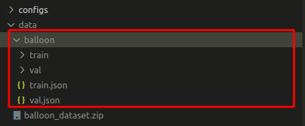
In this tutorial, we provide the ballon dataset, which is less than 40MB, as the training dataset for MMYOLO.

python tools/misc/download_dataset.py --dataset-name balloon --save-dir data --unzip
python tools/dataset_converters/balloon2coco.py

After executing the above command, the balloon dataset will be downloaded in the data folder with the converted format we need. The train.json and val.json are the annotation files in the COCO format.

Config File Preparation

Create a new file called the yolov5_s-v61_syncbn_fast_1xb4-300e_balloon.py configuration file in the configs/yolov5 folder, and copy the following content into it.

_base_ = './yolov5_s-v61_syncbn_fast_8xb16-300e_coco.py'

data_root = 'data/balloon/'

train_batch_size_per_gpu = 4
train_num_workers = 2

metainfo = {
    'classes': ('balloon', ),
    'palette': [
        (220, 20, 60),
    ]
}

train_dataloader = dict(
    batch_size=train_batch_size_per_gpu,
    num_workers=train_num_workers,
    dataset=dict(
        data_root=data_root,
        metainfo=metainfo,
        data_prefix=dict(img='train/'),
        ann_file='train.json'))

val_dataloader = dict(
    dataset=dict(
        data_root=data_root,
        metainfo=metainfo,
        data_prefix=dict(img='val/'),
        ann_file='val.json'))

test_dataloader = val_dataloader

val_evaluator = dict(ann_file=data_root + 'val.json')

test_evaluator = val_evaluator

model = dict(bbox_head=dict(head_module=dict(num_classes=1)))

default_hooks = dict(logger=dict(interval=1))

The above configuration is inherited from ./yolov5_s-v61_syncbn_fast_8xb16-300e_coco.py, and data_root, metainfo, train_dataloader, val_dataloader, num_classes and other configurations are updated according to the balloon data we are using. The reason why we set the interval of the logger to 1 is that the balloon data set we choose is relatively small, and if the interval is too large, we will not see the output of the loss-related log. Therefore, by setting the interval of the logger to 1 will ensure that each interval iteration will output a loss-related log.

Training

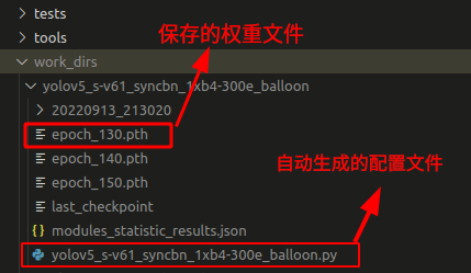
python tools/train.py configs/yolov5/yolov5_s-v61_syncbn_fast_1xb4-300e_balloon.py

After executing the above training command, the work_dirs/yolov5_s-v61_syncbn_fast_1xb4-300e_balloon folder will be automatically generated. Both the weight and the training configuration files will be saved in this folder.

Resume training after interruptions

If training stops midway, add --resume at the end of the training command, and the program will automatically load the latest weight file from work_dirs to resume training.

python tools/train.py configs/yolov5/yolov5_s-v61_syncbn_fast_1xb4-300e_balloon.py --resume

Fine-tune with loaded pretrained weights

NOTICE: It is highly recommended that finetuning from large datasets, such as COCO, can significantly boost the performance of overall network. In this example, compared with training from scratch, finetuning the pretrained model outperforms with a significant margin. (Over 30+ mAP boost than training from scratch).

1. Download the COCO dataset pre-trained weights

cd mmyolo
wget https://download.openmmlab.com/mmyolo/v0/yolov5/yolov5_s-v61_syncbn_fast_8xb16-300e_coco/yolov5_s-v61_syncbn_fast_8xb16-300e_coco_20220918_084700-86e02187.pth

2. Load the pretrained model to train

cd mmyolo
python tools/train.py configs/yolov5/yolov5_s-v61_syncbn_fast_1xb4-300e_balloon.py \
                      --cfg-options load_from='yolov5_s-v61_syncbn_fast_8xb16-300e_coco_20220918_084700-86e02187.pth'

3. Freeze backbone to train

Freeze the four backbone stages by setting model.backbone.frozen_stages=4 in the config file or from the command line.

# Set model.backbone.frozen_stages=4 from the command line
cd mmyolo
python tools/train.py configs/yolov5/yolov5_s-v61_syncbn_fast_1xb4-300e_balloon.py \
                      --cfg-options load_from='yolov5_s-v61_syncbn_fast_8xb16-300e_coco_20220918_084700-86e02187.pth' model.backbone.frozen_stages=4

Visualization

For visualization of default_hooks in configs/yolov5/yolov5_s-v61_syncbn_fast_1xb4-300e_balloon.py, we set draw to True and interval to 2.

default_hooks = dict(
     logger=dict(interval=1),
     visualization=dict(draw=True, interval=2),
)

Re-run the following training command. During the validation, each interval image will save a puzzle of the annotation and prediction results to work_dirs/yolov5_s-v61_syncbn_fast_1xb4-300e_balloon/{timestamp}/vis_data/vis_image folder.

python tools/train.py configs/yolov5/yolov5_s-v61_syncbn_fast_1xb4-300e_balloon.py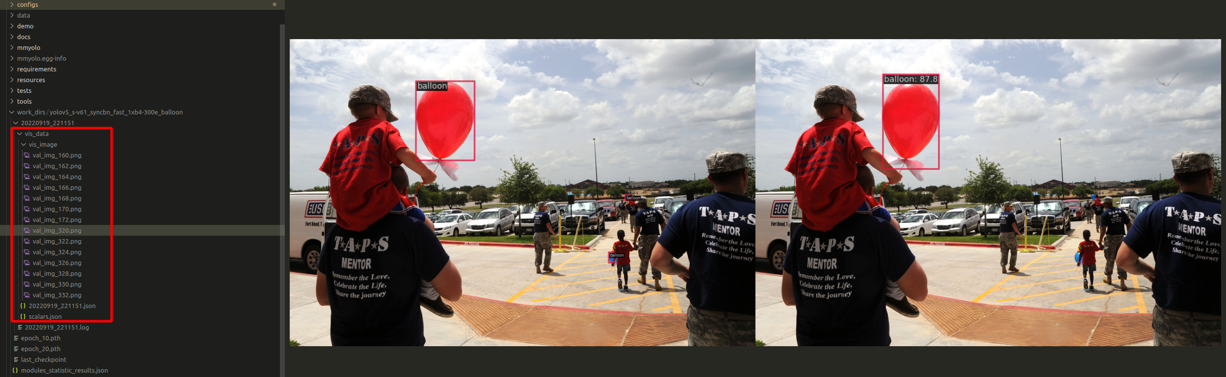

Visualization Backend Support

MMEngine supports various backends such as local, TensorBoard, and wandb.

• wandb

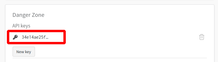
Register and get your wandb API key from the official website.

pip install wandb

wandb login
# enter your API key, then you can see if you login successfully

Add wandb configuration in configs/yolov5/yolov5_s-v61_syncbn_fast_1xb4-300e_balloon.py.

visualizer = dict(vis_backends = [dict(type='LocalVisBackend'), dict(type='WandbVisBackend')])

Re-run the training command to check data visualization results such as loss, learning rate, and coco/bbox_mAP in the web link prompted on the command line.

python tools/train.py configs/yolov5/yolov5_s-v61_syncbn_fast_1xb4-300e_balloon.py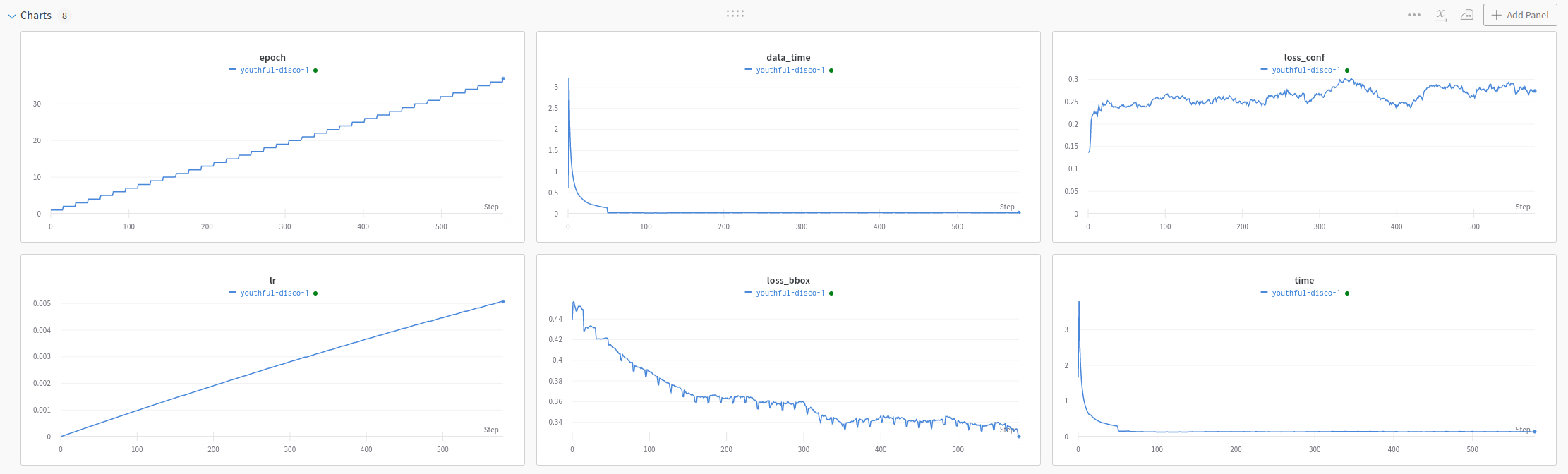

• Tensorboard

Install Tensorboard

pip install tensorboard

Similar to wandb, we need to add Tensorboard configuration in configs/yolov5/yolov5_s-v61_syncbn_fast_1xb4-300e_balloon.py.

visualizer = dict(vis_backends=[dict(type='LocalVisBackend'),dict(type='TensorboardVisBackend')])

Re-run the training command, a Tensorboard folder will be created in work_dirs/yolov5_s-v61_syncbn_fast_1xb4-300e_balloon/{timestamp}/vis_data, You can get data visualization results such as loss, learning rate, and coco/bbox_mAP in the web link prompted on the command line with the following command:

tensorboard --logdir=work_dirs/yolov5_s-v61_syncbn_fast_1xb4-300e_balloon

Model Testing

python tools/test.py configs/yolov5/yolov5_s-v61_syncbn_fast_1xb4-300e_balloon.py \
                      work_dirs/yolov5_s-v61_syncbn_fast_1xb4-300e_balloon/epoch_300.pth \
                      --show-dir show_results

Run the above command, the inference result picture will be automatically saved to the work_dirs/yolov5_s-v61_syncbn_fast_1xb4-300e_balloon/{timestamp}/show_results folder. The following is one of the result pictures. The left one is the actual annotation, and the right is the model inference result.

Model Deployment

Please refer to this