Jacques Thibodeau
October 31st, 2021
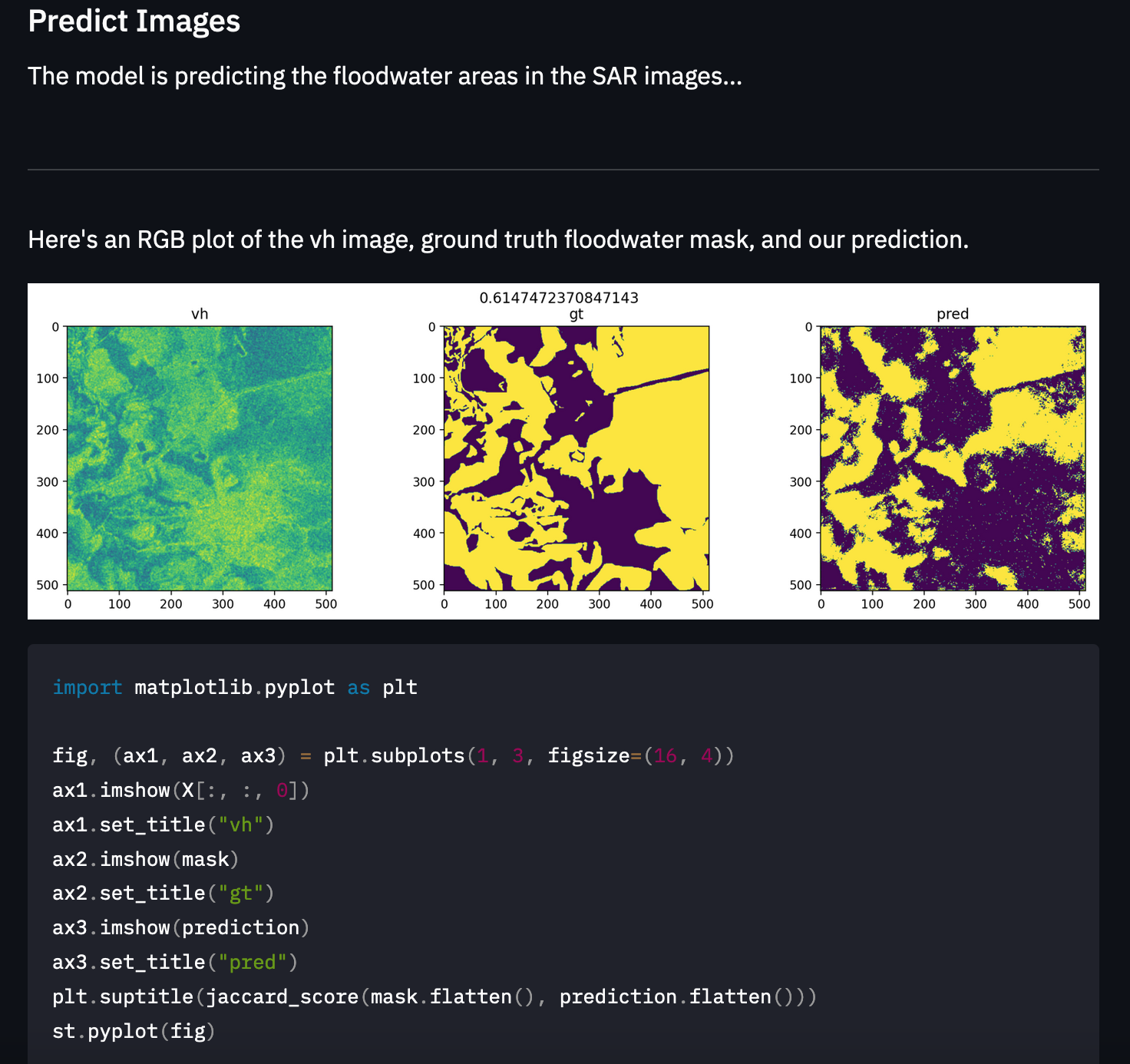
The Streamlit Web App that makes Predictions with SageMaker Model Endpoint:
Floods have always led to terrible tragedies. Over the centuries, humanity has learned to build infrastructure to prevent floods, yet many people still suffer and die from floods.
Another approach we can take in terms of prevention is to apply machine learning to predict when a flood is about to happen so that we can evacuate and protect ourselves sooner to mitigate the flooding impact. There are many approaches we can take to do this. However, one approach involves using satellite imagery to detect the presence of floodwater via semantic segmentation (classifying each pixel in an image as "does this pixel contain floodwater or not?").
This is easier said than done. We can use satellites with cameras operating in the visible wavelength range, but those images can be obscured by fog and clouds. One way to deal with this issue is to use cameras that take photos in the microwave wavelength band. The microwave wavelength band is not obscured by cloud and fog, and we can see right through them while still having a view of the Earth.
Each piece of land that the satellite's camera takes pictures of will have two images, one image in the VH polarization of light (vertical transmit and horizontal receive) and another in the VV polarization (vertical transmit and vertical receive). Both polarization brings out different characteristics in their images, allowing our model to learn all the intricacies of the land and better separate floodwater from non-floodwater.
In order to train our model to be able to separate floodwater from non-floodwater, we also have label masks that go with every pair of VV and VH images. So, our goal is to train a model that can map the VV and VH images to the label mask images where every pixel has been annotated as floodwater or non-floodwater.
As someone who is focused on using AI for good, this project is a great opportunity. As we improve our approach to predicting natural disasters before they happen, we can reduce suffering and save lives. It is crucial to act on this quickly due to the increasing impacts of climate change.
This project is an extension of the "STAC Overflow: Map Floodwater from Radar Imagery" competition on DrivenData.org: https://www.drivendata.org/competitions/81/detect-flood-water/page/386/
For this project, we are trying to build a machine learning model that can do semantic segmentation of floodwater to build a tool that provides us with early warnings that can help save lives and reduce damages from floods. This means that we are trying to separate the areas in an image where there is floodwater, and there is no floodwater.
We will be using synthetic-aperture radar (SAR) imagery to predict the presence of floodwater. This type of image data is different from typical image data. Therefore, the deep learning models typically used for image segmentation will not work well compared to regular RGB images. This is because the pre-trained models we are using for transfer learning were typically trained on a dataset with very few (or none) SAR images. In this case, we will be using pre-trained models (the backbone of our model) trained on imagenet, which does not have SAR images. For this reason, we can expect it will be much harder for our model to perform well.
We will use Unet and DeepLabV3 models with an encoder backbone model (ex: Resnet34) to do segmentation. We use this approach as it has been shown to perform exceptionally well on semantic segmentation tasks. We will be using the PyTorch Lightning and Segmentation Models (PyTorch) libraries to train our models. In order to get a good model, we will train two models with SageMaker's HyperparameterTuning feature and choose the best model for deployment.
Ultimately, our goal is to feed the model images in both the vh and vv polarizations and output a prediction of the floodwater locations in those images. We will not be too concerned about prediction performance since this project is about creating an end-to-end project with SageMaker, and it would cost too much money to train many models in SageMaker.
We will also build a Streamlit app to perform inference on the model endpoint with the SageMaker SDK.
So, we will:
- Do data exploration on the SAR images
- Preprocess the data
- Load data to S3
- Train models using SageMaker's HyperparameterTuning function (in the notebook, we commented out the hyperparameter tuning job to reduce runtime)
- Select the best model for deployment
- Deploy the model
- Perform inference on the deployed model in the notebook
- Perform inference on the deployed model in the Streamlit web app
Our goal is to get the highest performance on the Jaccard index metric (also known as Generalized Intersection over Union (IoU)). The Jaccard index measures the similarity between two label sets. In this case, it measures the size of the intersection divided by the size of the union of non-missing pixels. In other words, it measures how accurately we have segmented floodwater from other matter. If predicted segmentation matches exactly the ground truth, we will get a Jaccard index value of 1.0. The lower the value (down to 0), the lower the overlap between predicted and ground truth segmentation.

where A is the set of true pixels and B is the set of predicted pixels.
Ref (Performance metric): https://www.drivendata.org/competitions/81/detect-flood-water/page/386/
We will be using a subset of the Sentinel-1 dataset, which contains radar images stored as 512 x 512-pixel GeoTIFFs. In order to train our model to be able to separate floodwater from non-floodwater, we also have label masks that go with every pair of VV and VH images.
In GeoTIFFS, we have the image data as well as other metadata regarding the image, as we can see here:

This metadata gives us information like "nodata," which lets us know which values in the image are described as missing. In this case, all 0.0 values in the image are "missing values." We can also grab the bounding coordinates from the GeoTIFF (where was the image taken on Earth):

Along with the GeoTIFFs, we have a metadata CSV of the images that we use to identify each chip_id and its corresponding images of both polarizations.
The following quotes are from the DrivenData competition page (Training set - Images): https://www.drivendata.org/competitions/81/detect-flood-water/page/386/.
Each pixel in a radar image represents the energy that was reflected back to the satellite measured in decibels (dB). Pixel values can range from negative to positive values. A pixel value of 0.0 indicates missing data.
Sentinel-1 is a phase-preserving dual-polarization SAR system, meaning that it can receive a signal in both horizontal and vertical polarizations. Different polarizations can be used to bring out different physical properties in a scene. The data for this challenge includes two microwave frequency readings: VV (vertical transmit, vertical receive) and VH (vertical transmit, horizontal receive).

After looking at our data, there were no abnormalities we needed to fix in the dataset.
Note: we could have added additional data from the Microsoft Planetary Computer to augment our dataset with information about things such as elevation, but we need to ask for special permission from Microsoft to have access. We gained access, and we could work with the data in Colab, but we left it out of SageMaker since the project reviewer will not have access.
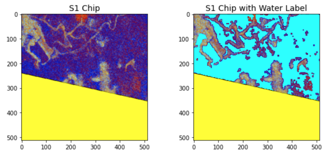
Since the images are not taken in the human visible wavelength range, we need to apply a false-colour composite to visualize the images. However, this is only for visualization; we will not use the false-colour composite images as training data.
VV Polarization example:

VH Polarization example:

Each image has a chip_id associated with it. There is

Notice how some countries have a lot more chips than others. We will not be taking this into account for our model, but we could imagine that some images will be more common in the dataset than others. Therefore, it may be that the model performs well on US data (for example) but performs poorly on Bolivia data since it simply does not have enough data for that kind of terrain. If we wanted to fine-tune the model further, we could identify the types of locations where the model performs poorly and improve those kinds of terrains. For example, we could create a specialized model for that data and include it in an ensemble. We could also find those types of images and pre-train a model before fine-tuning it.
Pixel values represent energy that was reflected back to the satellite measured in decibels. To better visualize the bands or channels of Sentinel-1 images, we will create a false-colour composite by treating the two bands and their ratio as red, green, and blue channels, respectively. The yellow indicates missing values. The teal blue in the right image indicates the water label mask we are trying to predict.
Our task is to do semantic segmentation of satellite-aperture radar imagery in order to classify each pixel in an image as to whether it contains floodwater or not. The state-of-the-art techniques in this domain involve using a deep learning model where the first portion of the neural network (the backbone/encoder) is a pre-trained model like ResNet34. Then, we attach a Unet-like architecture to the output of the backbone model.
This is what a Unet architecture looks like:

A U-Net architecture is divided into two parts: the contracting part, which follows the typical CNN architecture, which downsamples for classification, followed by an expansive part that upsamples the feature map to an output segmentation map. The second part is crucial for segmentation because, in image segmentation, we need to convert the feature map into a vector and reconstruct the image from this vector so that we can segment the image.
When training our model, we will focus on three different configuration changes to improve our model: model architecture (Unet or other model heads like DeepLabV3, UnetPlusPlus, DeepLabV3Plus), backbone model (ResNet34, EfficientNet-b0, xception), and learning rate (0.001, 0.0003, 0.0001). We did several hyperparameter tuning jobs with a combination of all of those configuration possibilities.
To feed the image data to our model, we first have to stack the arrays of the VH and VV images together. Then, we apply a min-max normalization on the input pixel values (unique for our dataset; makes sure we have no negative values and normalizes across pixels), apply data augmentations with the Albumentations package (ex: RandomCrop, RandomRotate90, HorizontalFlip, and VerticalFlip), and then pass those values to our model for training.
We wanted to try creating a final ensemble model of the best models, but it was a bit too complicated to do in SageMaker and was not worth the effort.
For the benchmark, we can start by looking at the benchmark from the blog post of the competition: https://www.drivendata.co/blog/detect-floodwater-benchmark/.
The blog post ended up with a validation IOU of 0.3069. We ended up with 0.32162. Perhaps this was because we trained if for longer. We will use our performance of 0.32162 as the benchmark.
The benchmark model is a U-Net model with a ResNet34 as the backbone of the model. This model performs well in most cases when it comes to semantic segmentation tasks. This is because the model starts as a typical vision model as the backbone (in this case, ResNet34), and then that serves as input to the remaining layers, which are in a U-Net architecture. This type of model is often what people use when starting a semantic segmentation project, and they want to build an end-to-end pipeline quickly. Therefore, it is the perfect model to choose as a benchmark.
Before model training, we need to prepare the data in a specific way.
First, we split the data (with a random seed) to create a training set and a validation set. Then, we create a dataframe where each row describes a chip_id, which links to the set of VH and VV images. We need to make sure that the path to the training files is properly created in the dataframe. Since our model is trained in a Docker container, we need to set the filepaths to the paths the dataset will be downloaded to in the Docker container. This is in the /opt/ml/input/data/data_s3_uri/ subdirectory.
To feed the image data to our model, we read the images as NumPy arrays and then we have to stack the arrays of the VH and VV images together. Then, we apply a min-max normalization on the input pixel values (unique for our dataset; makes sure we have no negative values and normalizes across pixels), apply data augmentations with the Albumentations package (ex: RandomCrop, RandomRotate90, HorizontalFlip, and VerticalFlip), and then pass those values to our model for training.
In the notebook, we have the option of either training a single model with Estimator.fit() or training multiple models with HyperparameterTuner. We trained models with both methods.
In the case of the HyperparameterTuner, we need to pass the hyperparameters for our models in a special way. We start by choosing which hyperparameters we want to tune by giving that hyperparameter more than one option. For example, we wanted to test out which architecture would perform the best, so we gave it model two choices:
hyperparameter_ranges = {"architecture": CategoricalParameter(["Unet", "DeepLabV3"])}
And then, we create another dictionary containing the hyperparameters that will not be changing during the tuning job:
hparams = {
"backbone": "efficientnet-b0",
"weights": "imagenet",
"lr": 1e-3,
"min_epochs": 6,
"max_epochs": 40,
"patience": 5,
"batch_size": 8, # reduce batch_size if you get CUDA error
"num_workers": 8,
"val_sanity_checks": 0,
"output_path": "model-outputs",
"log_path": "tensorboard_logs"
}
Once we have all of those values, we can include it in the HyperparameterTuner object to instantiate our tuner:
tuner = HyperparameterTuner(
estimator,
objective_metric_name,
hyperparameter_ranges,
metric_definitions,
max_jobs=2,
max_parallel_jobs=1,
strategy="Random",
objective_type=objective_type,
base_tuning_job_name='floodwater-tuning'
)
Once we have our tuner, we can call tuner.fit() by passing the inputs:
inputs = {'data_s3_uri': data_s3_uri, 'train_features': features_path, 'train_labels': labels_path}

tuner.fit(inputs=inputs, wait=True)
When writing a train.py file for hyperparameter tuning in SageMaker, we need to be careful about passing our hyperparameters to the model. For example, if we have passed the hyperparameters to HyperparameterTuner, then we need to parse the hyperparameters for training like so:
## Below is only used when we are running a Hyperparameter Tuning job.

# hyperparameters sent by the client are passed as command-line arguments to the script.
parser.add_argument('--architecture', type=str, default=os.environ['SM_HP_ARCHITECTURE'])
parser.add_argument('--backbone', type=str, default=os.environ['SM_HP_BACKBONE'])
parser.add_argument('--weights', type=str, default=os.environ['SM_HP_WEIGHTS'])
parser.add_argument('--lr', type=float, default=os.environ['SM_HP_LR'])
parser.add_argument('--min_epochs', type=int, default=os.environ['SM_HP_MIN_EPOCHS'])
parser.add_argument('--max_epochs', type=int, default=os.environ['SM_HP_MAX_EPOCHS'])
parser.add_argument('--patience', type=int, default=os.environ['SM_HP_PATIENCE'])
parser.add_argument('--batch_size', type=int, default=os.environ['SM_HP_BATCH_SIZE'])
parser.add_argument('--num_workers', type=int, default=os.environ['SM_HP_NUM_WORKERS'])
parser.add_argument('--val_sanity_checks', type=int, default=os.environ['SM_HP_VAL_SANITY_CHECKS'])
parser.add_argument('--log_path', type=str, default=os.environ["SM_HP_LOG_PATH"])
However, for this project, there is something that causes an error if we pass it as a "hyperparameter", which is the training metadata dataframe. Because our training is done in a Docker container outside the SageMaker notebook, we cannot simply pass our training data as a "hyperparameter" as we can in Colab or another notebook that does not use Docker. So why would we want to pass the training data as a "hyperparameter" anyways? It is easier. We can pass a dataframe inside of a python dictionary in a regular notebook, but we cannot do that when doing a training run in SageMaker. That is why we need to load the training metadata dataframe inside the train.py file and then add it to the hparams dictionary for training.
We are using the segmentation_model.pytorch package to fine-tune some pre-trained models. In order to train different types of model with our HyperparameterTuner, I needed to instantiate the model like this:
cls = getattr(smp, self.architecture)
model = cls(
   encoder_name=self.backbone,
   encoder_weights=self.weights,
   in_channels=2,
   classes=2,
)
In other words, we grab either architecture with getattr(smp, self.architecture) and then instantiate it with cls(...).
Now that we have an instantiated model, we can put it in the PyTorch Lightning LightningModule, making it easy to train a PyTorch model. Of course, there is a lot to know about Lightning, but it essentially works by removing all the boilerplate code of pure PyTorch, making it easier to train a model and less bug-prone. In addition, it has specific methods that make training simpler.
If we focus on the training part, we see in training_step that our model starts by grabbing each batch of images passed to our model. Those batches are pixel arrays of our images passed to the model. x is our training images, and y' is what we are training to predict (our ground truth). Next, we have our images go through the forward method, which takes the input images and calculates the prediction (preds`) after going through the model's layers.
def forward(self, image):
    # Forward pass through the network
    return self.model(image)

def training_step(self, batch, batch_idx):
    # Swtich on training mode
    self.model.train()
    torch.set_grad_enabled(True)

    # Load images and labels
    x = batch["chip"]
    y = batch["label"].long()
    if self.gpus:
        x, y = x.cuda(non_blocking=True), y.cuda(non_blocking=True)

    # Forward pass
    preds = self.forward(x)

    # Calculate training loss
    criterion = XEDiceLoss()
    xe_dice_loss = criterion(preds, y)
    print('Successfully calculated loss.')

    # Log batch xe_dice_loss
    self.log(
        "xe_dice_loss",
        xe_dice_loss,
        on_step=True,
        on_epoch=True,
        prog_bar=True,
        logger=True
    )

    return xe_dice_loss
We keep going through each batch of the data. Once we have gone through all the batches, we have finished the epoch, and we can calculate the model performance by seeing how well it performs on the validation data.
The most significant change we did after training several models was to use EfficientNet-b0 as the backbone model instead of a ResNet34.
A loss function is what we use in deep learning to help our model know how well it is performing and, by consequence, how we should update the model weights. We used the XEDiceLoss loss function to train our model. From the Benchmark Blog Post of the competition:
For training, we will use a standard mixture of 50% cross-entropy loss and 50% dice loss, which improves learning when there are unbalanced classes. Since our images tend to contain more non-water than water pixels, this metric should be a good fit. Broadly speaking, cross-entropy loss evaluates differences between predicted and ground truth pixels and averages over all pixels, while dice loss measures overlap between predicted and ground truth pixels and divides a function of this value by the total number of pixels in both images. This custom class will inherit torch.nn.Module, which is the base class for all neural network modules in PyTorch. A lower XEDiceLoss score indicates better performance.
When we used earlier versions of torch, I had many issues with this loss function. This was because the dtypes for torch.where() used to have to be very particular. However, when we switched to using more recent versions of torch, I no longer had any data type errors.
That said, I did need to add .float() to self.xe(pred, temp_true).float() because I could not calculate the mean of xe_loss.masked_select(valid_pixel_mask).mean() without it.
class XEDiceLoss(nn.Module):
"""
Computes (0.5 * CrossEntropyLoss) + (0.5 * DiceLoss).
"""

def __init__(self):
    super().__init__()
    self.xe = nn.CrossEntropyLoss(reduction="none")

def forward(self, pred, true):
    valid_pixel_mask = true.ne(255) # valid pixel mask

    # Cross-entropy loss
    temp_true = torch.where((true == 255), 0, true) # cast 255 to 0 temporarily
    xe_loss = self.xe(pred, temp_true).float()
    xe_loss = xe_loss.masked_select(valid_pixel_mask).mean()

    # Dice loss
    pred = torch.softmax(pred, dim=1)[:, 1]
    pred = pred.masked_select(valid_pixel_mask)
    true = true.masked_select(valid_pixel_mask)
    dice_loss = 1 - (2.0 * torch.sum(pred * true)) / (torch.sum(pred + true) + 1e-7)

    return (0.5 * xe_loss.long()) + (0.5 * dice_loss)
We used the same performance metric (Jaccard index / Intersection Over Union) as the blog post to evaluate our model. Again, there were no issues with it.
We ran into many issues when trying to train the models. So we will go through them here.
CUDA Error: If you are getting a CUDA error that says something like "CUDA_ERROR_ILLEGAL_ADDRESS: an illegal memory access was encountered.", this can likely be resolved by reducing the batch_size. For example, we were using batch_size of 32 with ml.p2.xlarge, and the model was training fine, but when we started using ml.p3.2xlarge, we kept getting that error. It was only after we reduced the batch_size to 8 that we were able to resolve the issue.
Using big models: We might also get a CUDA error using a different model architecture. The bigger the model, the more likely this will happen since we will not be able to store all the model weights in memory. We focused on using simpler models in SageMaker, so this issue did not come up often.
Wrong dtype in our tensors: If we get an error like Expected Float but got Long, it likely is an issue with our torch version. The older version will often have this issue, and we will notice it for CrossEntropy calculations. Therefore, either install a newer version so that we have to worry about that less or make sure to convert our tensors to the correct data types for the operations we want to do on them. For example, CrossEntropy needs to have float values in older torch versions. There are also some specific methods like calculating the tensor Mean that need to have a tensor of floats rather than Long.
To make sure that we save the best model after training, we need to add the following code to the train.py file:
# Runs model training
ss_flood_model.fit() # orchestrates our model training

best_model = FloodModel(hparams=hparams)
best_model_path = ss_flood_model.trainer_params["callbacks"][0].best_model_path
best_model = best_model.load_from_checkpoint(checkpoint_path=best_model_path)

# After model has been trained, save its state into model_dir which is then copied to back S3
with open(os.path.join(args.model_dir, 'model.pth'), 'wb') as f:
    torch.save(best_model.state_dict(), f)
The "best model" is the checkpointed model based on the best performance on our performance metric (validation IOU). If we do not save the best model correctly, we end up saving the last epoch of our model, which could mean that we are saving a model that is overfitting or does not have as good model weights as the best checkpointed model.
To deploy a PyTorch model in SageMaker, we need to create four special methods that SageMaker recognizes:
- The
model_fnmethod needs to load the PyTorch model from the saved weights from disk. - The
input_fnmethod needs to deserialize the invoke request body into an object we can perform prediction on. - The
predict_fnmethod takes the deserialized request object and performs inference against the loaded model. - The
output_fnmethod takes the result of prediction and serializes this according to the response content type.
Source for above: https://course19.fast.ai/deployment_amzn_sagemaker.html
Here is the serve/inference.py script:
    import json
    import torch
    import numpy as np
    import os
    from io import BytesIO

    from model import FloodModel


    def model_fn(model_dir):
        print("Loading model...")
        model = FloodModel()
        with open(os.path.join(model_dir, 'model.pth'), 'rb') as f:
            model.load_state_dict(torch.load(f))
            print("Finished loading model.")
        return model


    def input_fn(request_body, request_content_type):
        print("Accessing data...")
        assert request_content_type == 'application/x-npy'
        load_bytes = BytesIO(request_body)
        data = np.load(load_bytes, allow_pickle=True)
        print("Data has been stored.")
        return data


    def predict_fn(data, model):
        print("Predicting floodwater of SAR images...")
        with torch.no_grad():
            prediction = model.predict(data)
        print("Finished prediction.")
        return prediction


    def output_fn(predictions, content_type):
        print("Saving prediction for output...")
        assert content_type == 'application/json'
        res = predictions.astype(np.uint8)
        res = json.dumps(res.tolist())
        print("Saved prediction, now sending data back to user.")
        return res
We also need to create a special inference version of our PyTorch model to instantiate it in model_fn and call it in predict_fn. For this, we created the serve/model.py script:
import numpy as np
import torch
import pytorch_lightning as pl
import segmentation_models_pytorch as smp
import os

pl.seed_everything(9)

class FloodModel(pl.LightningModule):
    def __init__(self):
        super().__init__()
        print("Instantiating model...")
        self.architecture = 'Unet' # os.environ['SM_MODEL_ARCHITECTURE']
        self.backbone = "efficientnet-b0"
        cls = getattr(smp, self.architecture)
        self.model = cls(
           encoder_name=self.backbone,
           encoder_weights=None,
           in_channels=2,
           classes=2,
        )
        print("Model instantiated.")

    def forward(self, image):
        # Forward pass
        print("Forward pass...")
        return self.model(image)

    def predict(self, x_arr):
        print("Predicting...")
        # Switch on evaluation mode
        self.model.eval()
        torch.set_grad_enabled(False)

        # Perform inference
        preds = self.forward(torch.from_numpy(x_arr))
        preds = torch.softmax(preds, dim=1)[:, 1]
        preds = (preds > 0.5) * 1
        print("Finished performing inference.")
        return preds.detach().numpy().squeeze().squeeze()
We had an issue with passing environment variables to the deployed endpoint. We wanted to create a notebook that could train multiple models, take the best model, and then pass environment variables that help recreate the best model (architecture) to the inference endpoint. Unfortunately, we could not figure this out since the SageMaker documentation on inference is quite bad, and we could not get in touch with anyone at AWS who could help.
We looked at the CloudWatch logs to figure things out, and the closest we could get was to make sure to add SM_HP_ when using os.environ[SM_HP_{hyperparameter}], but even that did not work.
Once the model has been deployed, we can send data to the model endpoint for prediction. When sending data to the endpoint with predictor.predict(data), we need to make sure that we properly serialize and deserialize the data. This was a big issue for this project because our image data was too big to be sent via JSON. When converting a NumPy ndarray into a JSON, the size of the data increases. In SageMaker, there is a limit of 5 MB that can be sent per request. When sent as a JSON, our data was closer to 10 MB, so we could not send the data in that format. We also had a hard time sending the data as a pure GeoTIFF image because the serialization methods in SageMaker only allow for JPEG, PNG or "application/x-image" (which also did not work). We did not think it would be wise to convert the GeoTIFFs in another image format.
Luckily, we have a few different serialization options in SageMaker (and worst case, we can create our custom serializer). After trying multiple different serialization approaches, we realized that the best approach was to use the NumpySerializer and the JSONDeserializer. That means that our data is sent to the endpoint as a NumPy ndarray, and then we need to make sure to convert the predictions as JSON before sending it back. We were lucky that there was no issue with using JSONDeserializer.
This is how we deployed the model:
from sagemaker.serializers import NumpySerializer
from sagemaker.deserializers import JSONDeserializer
predictor = inference_model.deploy(
    initial_instance_count=1,
    instance_type=instance_type,
    endpoint_name=endpoint_name,
    serializer=NumpySerializer(),
    deserializer=JSONDeserializer(),
    wait=True,
)
Before sending the data for prediction, we do all the preprocessing necessary to convert the two polarized images into a single NumPy ndarray.
Finally, we want to note that we also created a web app that could interact with the endpoint and receive prediction results. We used the SageMaker Python SDK to send requests to the endpoint rather than setting up a Lambda Function with API Gateway. After setting up my AWS credentials on my local machine, I can send requests to the endpoint by simply calling:
predictor = Predictor(
    ENDPOINT_NAME,
    serializer=NumpySerializer(),
    deserializer=JSONDeserializer(),
)
We started by training a model using the same configuration as the Benchmark blog post:
- Architecture: Unet
- Encoder/Backbone model: ResNet34
- Learning Rate: 0.001
The blog post ended up with a validation IOU of 0.3069. We ended up with 0.32162. Perhaps this was because we trained if for longer.
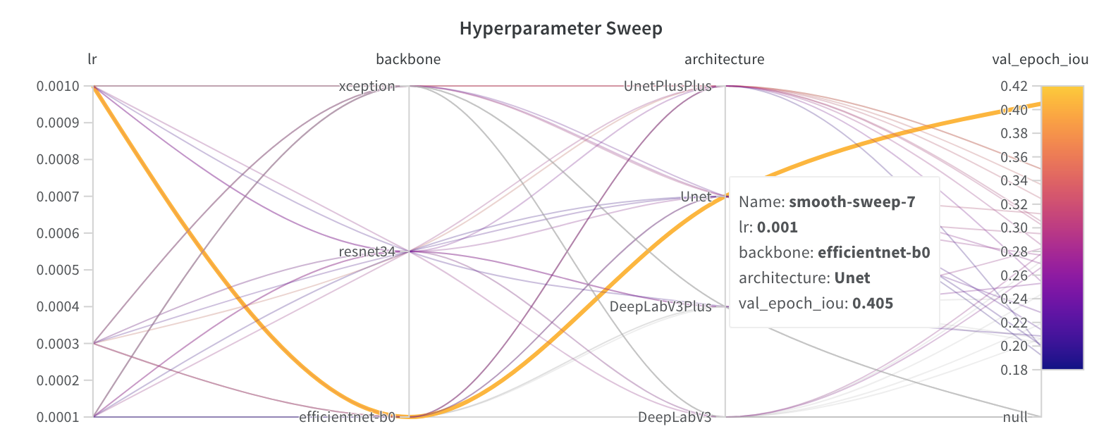
Afterwards, we wanted to tune the hyperparameters, so we trained many models in SageMaker using the Hyperparameter Tuning feature and in Google Colab (we used Weights and Biases to train the models), and we found that the best configuration for our model is the following:
(Best model configuration found using a Weights and Biases Hyperparameter Sweep in Google Colab)
- Architecture: Unet
- Encoder/Backbone model: EfficientNet-b0
- Learning Rate: 0.001
This gave us a validation IOU (our comparison metric) of 0.405 in Colab, which is much better than what was obtained in the benchmark blog post (0.3069).
Here are the results of the hyperparameter sweep we ran with Weights and Biases; the selected hyperparameter curve shows our best model:
We also tried different data augmentation configurations, but we were not getting better results, so we stuck with the ones I have.
Final Model: Our final model that we trained in SageMaker got us a validation IOU of 0.435 (using the same parameters as the best Colab model), much higher than the benchmark.
After training several models via hyperparameter tuning, we ended up choosing the Unet+EfficientNet-b0 architecture for our model. This model performed the best on the validation set, so that is why we chose it.
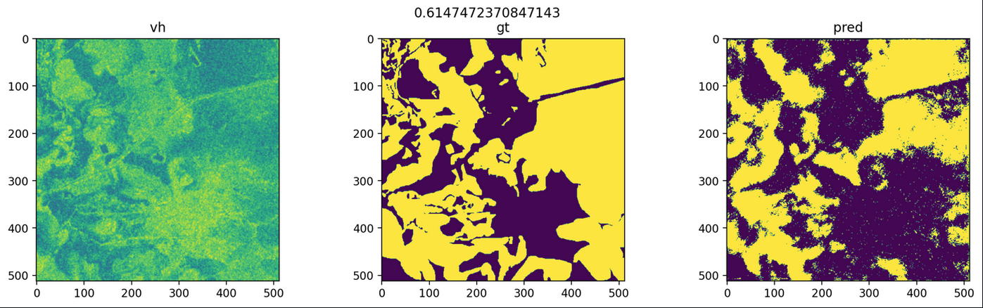
After looking at the results of a few images, we have noticed that the model is good at predicting floodwater if there is a whole lot in the image. However, it is not always accurate at predicting the correct shape of the floodwater. If there is not much floodwater in the image or it is not too prominent, it can miss the floodwater.
As we can see here, the model did a reasonably great job at predicting the floodwater and its shape:
Image 1
However, we can see in this image that while the model got a decent IOU score (Intersection Over Union), but it is just assuming that there is floodwater everywhere:
Image 2
The model seems good at knowing if there is much floodwater but still needs improvement at figuring out the shape of the floodwater.
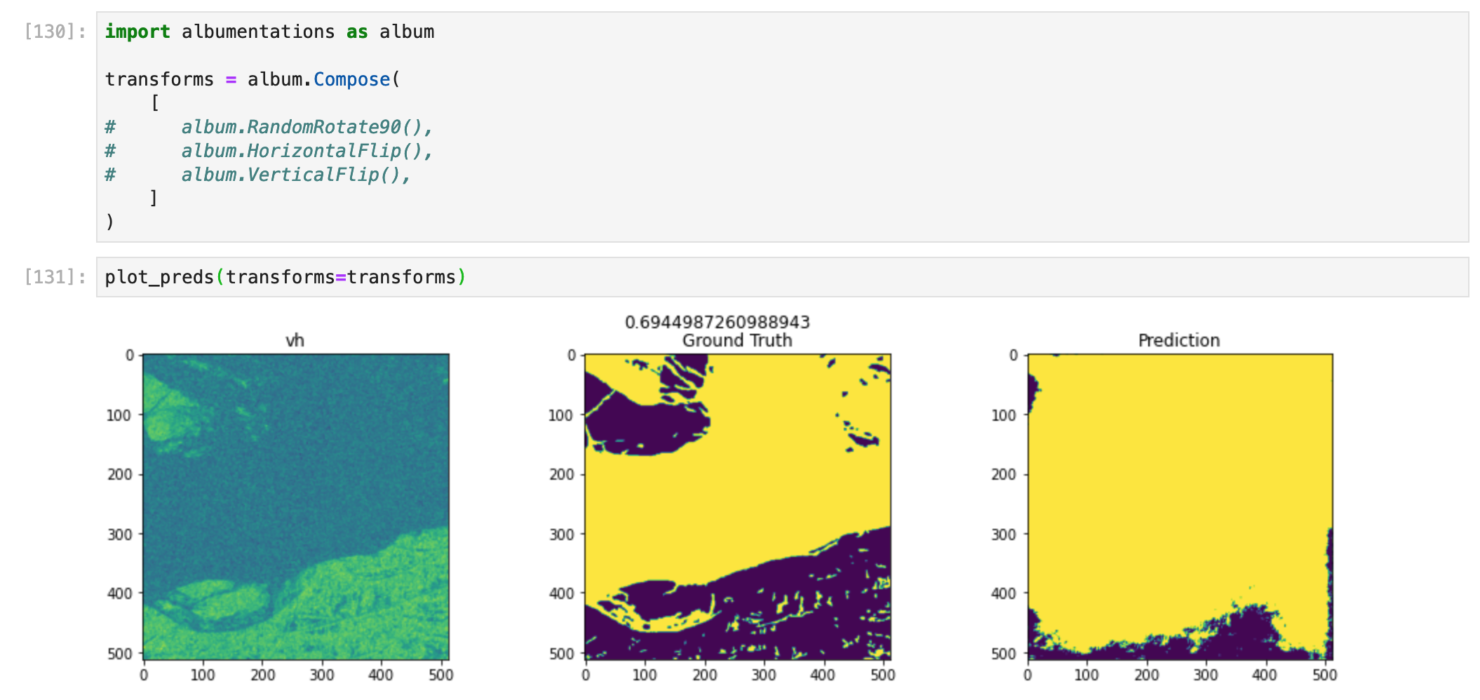
Below is an example of an image with very little floodwater. The model is quite bad at detecting these faint signs of floodwater:
Image 3
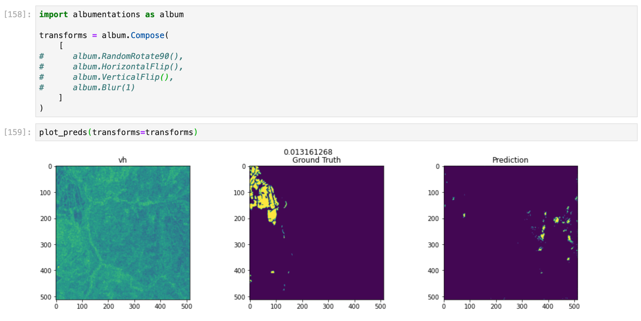
Image 2 and 3 were tested after applying data transforms. The results are in the following section.
To check our model's performance, we created a test set to evaluate the model after training. We do not have access to the competition test set, so we had to take away from the validation set to create a small test set. The model was not performing as well on the test set as it was on the validation set. There is definitely improvement needed so that the model can do just as well on unseen data. Our final model got the following results (better in both cases as the benchmark blog post):
- Validation set: 0.435
- Test set: 0.31045
We also added data transformations to the test images to see how well the model would perform if we did some basic alterations, like flipping it vertically using the albumentations package. Our model will usually perform worse after such transformations or perform just as well as without any transformation. Below are a few examples where we test our model's performance while using these transformations:
Image 2, no transforms.
Image 2, vertical flip. Performance doesn't change.
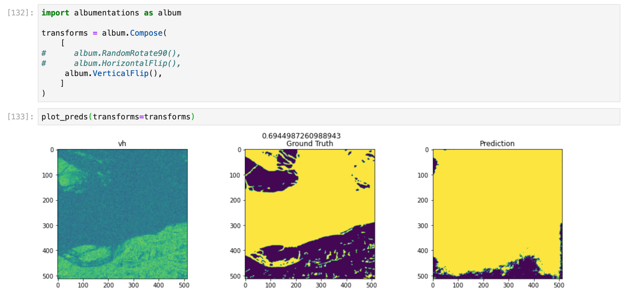
Image 2, horizontal and vertical flip. Performance is lower, and floodwater shape changed.
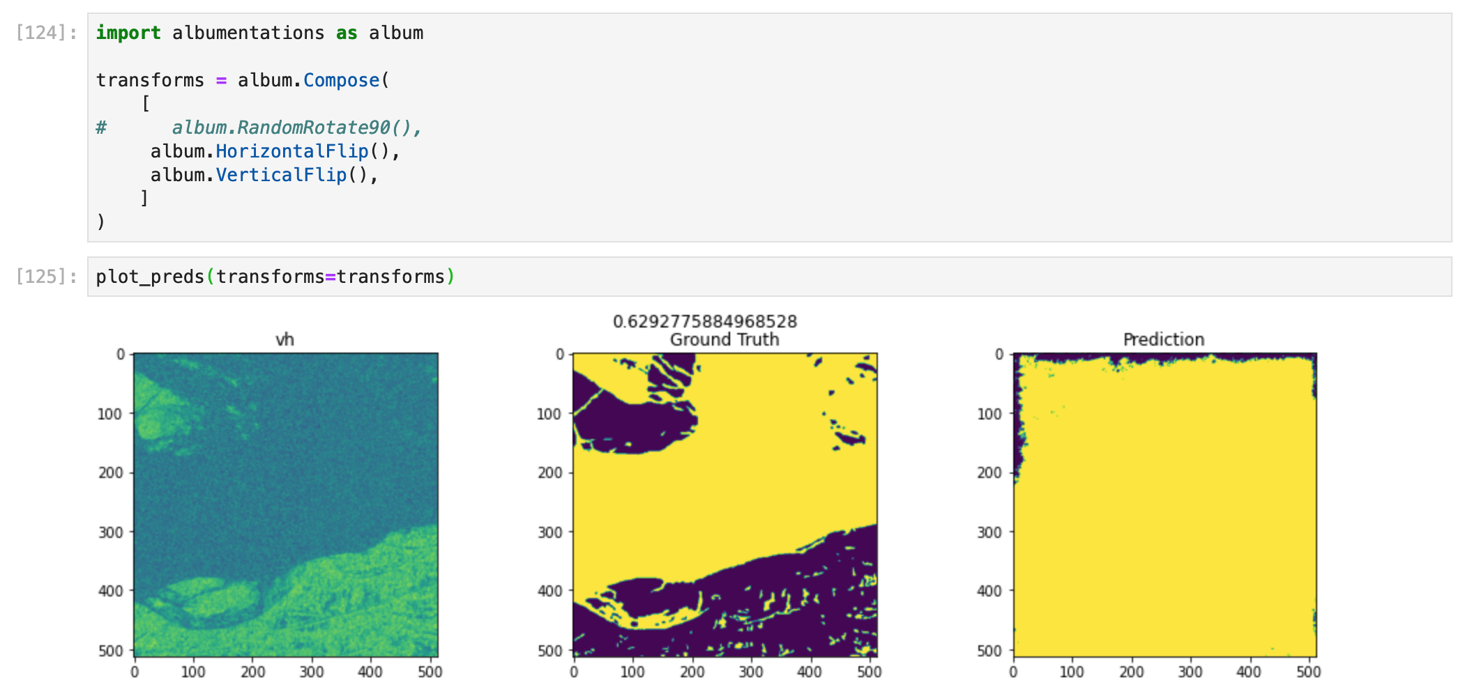
Image 3, no transforms.
Image 3, 90 degree rotation.
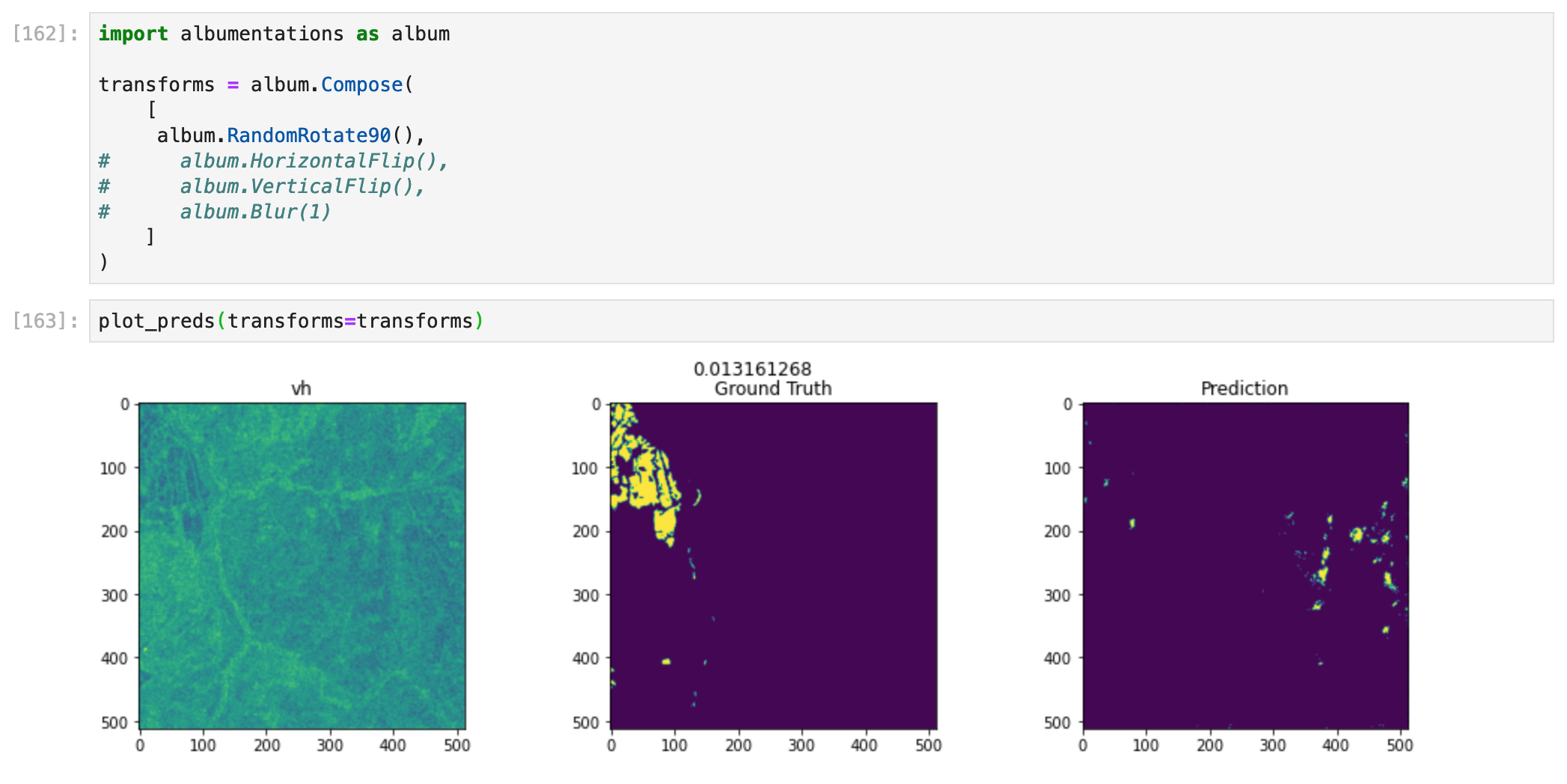
Image 3, vertical flip. Performance is lower, but it was already low, to begin with.
Not really. There is still much improvement left to do on this project, but that is also expected since this is a difficult problem. We have some ideas I could not implement while doing this project that could improve the performance and robustness of the model; we mention those in conclusion. We would not put this model in production until the model performance has improved. The only thing we would say is that the model might be decent enough to detect significant amounts of floodwater and if there is no floodwater at all. If this is the case, the model may be good enough depending on how crucial it is to predict the floodwater shape accurately. Nevertheless, it still needs improvement at figuring out the shape of the floodwater and detecting more obscure and small amounts of floodwater.
As we said in the Refinement section, the benchmark blog post got a validation IOU of 0.3069. On our first hyperparameter tuning run, our best benchmark model ended up with a validation IOU of 0.32162. The higher performance may be because of longer training time.
Our best and final model got a validation IOU of 0.435. Since our final model is performing better than the benchmarks, we can be happy with that result.
As we said in the previous section, this model will have to do for this project. There could certainly be some improvements (which we will mention in the conclusion), but after checking how our model performs, we can only say that whether we use the model will depend on our problem. For example, it may be that we only want a production model that can at least figure out if there is more than x% of floodwater in the image, meaning that we use the model to classify whether there is a lot of floodwater or none.
If we want to predict where exactly floodwater is via satellite imagery, we would need to improve the model.
All in all, we were able to build a decent model with an end-to-end notebook. However, since this is a difficult task still being researched, we could not expect +99% accuracy like we would for a cats and dogs classifier.
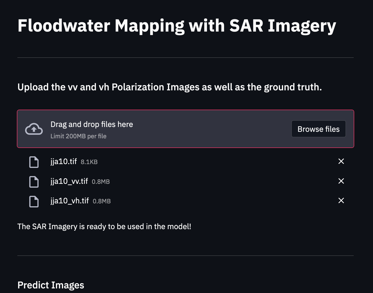
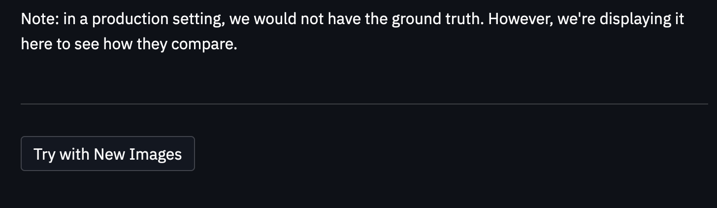
As was shown in the results section, we created a web app that can send a request to the endpoint and get back a prediction. In addition, the web app provides us with a visualization of the prediction result, which is quite helpful to actually see the predicted floodwater.
If we were to use this model in a company, we would want to have a real-time version of this visualization (minus the ground truth since we would not have one) to pinpoint where there is flooding and then act accordingly.
We will start by going over the entire end-to-end project.
Preparing the data for SageMaker
We first needed to download the images and metadata from the Driven Data Competition and upload it to S3 as a zip file to prepare the data. Once the data was stored, we could download the data into our SageMaker workspace and start working with the data.
We were then able to explore the data and better understand the properties of the GeoTIFF format. Next, we looked at the particulars of the project data and then moved on to prepare the data for model training.
To prepare the data, we split the dataset into training, validation, test sets and then uploaded those files along with the metadata file that contains the filepaths for the images.
Preparing the training code for use in SageMaker
To prepare the model, we had to create several files for training:
- We created the
train.pyfile to grab the hyperparameters that will be used for training, grab the data, fit the model, and then save the best model. - We created the
dataset.pyfile, which prepares and loads the torch data onto GPU for model training. - We created the
model.pyfile that contains the model we use for training. The model used depends on what we choose. We used thesegmentation_models.pytorchto easily create state-of-the-art segmentation models. To build the model, we used PyTorch Lightning since it removes all the boilerplate code that comes with pure PyTorch and just makes training a lot easier and less bug-prone. - We created the
loss_functions.pyfile because our model needs a loss function to update its model weights. We used a custom loss function that combines Binary Cross-Entropy Loss and Dice Loss. - We created the
metrics.pyto measure the model's performance. This is the metric that is human-understandable. We used the Intersection Over Union metric (Jaccard index) to measure model performance. - We created the
requirements.txtfile so that the Docker container used to train our model in SageMaker can properly install all the packages we need for training.
Training 2 models using HyperparameterTuning and choosing the best model
Instead of only training one model, we decided to use the SageMaker HyperparameterTuning feature to train multiple models by passing the sets of hyperparameters we would like to train the model on. Once the models are trained, we can look at the results and choose the best model.
Note: we also trained many models in Google Colab to save on compute costs in SageMaker. We trained those models using Weights and Biases since it allowed us to easily do a hyperparameter tuning job (they call them hyperparameter sweeps).
Doing inference on the image (.tif) data
To do inference, we needed to create a special inference.py file that allows the deployed endpoint to use PyTorch for inference. We also needed to create a new model.py file which contained an inference version of the model we created for training. The inference model contains a predict method and does not bother including all other special methods that come with PyTorch Lightning.
After setting up the serve directory, we deployed the model and got predictions from the model in the notebook and with the Streamlit app we created.
We needed to ensure that the data was correctly prepared and could be serialized to the endpoint and then deserialized from it for the predictions to work. So, instead of sending the examples for predictions as images or a JSON, we send the data as a Numpy ndarray of the pixel data.
Once a prediction is returned, we can plot the results of the predicted image to see how well it did visually.
Creating a Streamlit app to do inference
As an addition to the notebook, we created a Streamlit app that can be used to load images we want to predict, send a request to the deployed model endpoint, and then get back the predicted floodwater image. Here is what the app looks like:

Difficult Aspects
There were quite a few difficulties I came across during this project. However, the most unique one for this particular project was that we were working with GeoTIFFs. Those are images that are difficult to work with when doing inference in SageMaker.
First of all, we needed to send two images for one prediction, so we needed to get a bit creative about how we wanted to send the data to the endpoint. SageMaker seems only to allow users to send one image at a time. We can send batches to get batch inference, but that is different from sending two images for one prediction. Even if we wanted to send the image data to the endpoint, SageMaker does not support the GeoTIFF file format.
Then, when we wanted to convert the images into JSON for inference, the images were too big in size and therefore, the JSON had too many bytes to be sent to the endpoint (SageMaker has a limit).
Ultimately, we solved this problem by sending the data as a Numpy ndarray. We needed to stack the pixel data from both images to send as one piece of data.
Does this solution meet expectations?
If we were to actually deploy a model like this in a live production setting, we would want to spend some more time improving the model first. The following steps would be to add supplementary data and create an ensemble model. A project that gets us an end-to-end solution is exactly what we were expecting, and we learned a lot.
To improve our model performance results, we can do some of the following things:
- Use an ensemble of the models (we tried to do this but deployed ensembles are a little complicated in SageMaker, and the documentation is not too clear, so we decided we would only deploy a single model).
- If we use an ensembled model, we can decide to use the max value of either model in the ensemble since this will bias towards predicting floodwater. Based on our predictions from the model, it seems that the model is more likely to miss predicting floodwater over non-floodwater. Therefore, it would make sense to choose the max if one of the models predicts floodwater and another one (incorrectly) is not.
- The models added to the ensemble could also be something like a CatBoostedClassifier that predicts every pixel. From their website: "CatBoost is a machine learning algorithm that uses gradient boosting on decision trees."
- Train many more models using different albumentations, backbone models, architectures (head), and loss functions.
- We could use the additional data from Microsoft Planetary Computer. In particular, the Nasadem band is incredibly important. It is also worth pointing out that we did try also installing GDAL to the SageMaker notebook (it is needed to add the additional data). However, we would have needed to fiddle with the AWS environment. This would have led to a long installation time for the reviewer and additional steps (we would not be able to run the notebook simply).
- We could pre-train a deep learning model on Satellite-Aperture Radar (SAR) images because the current backbone/encoder models used in Semantic Segmentation are pre-trained on imagenet (a large image dataset), which does not have SAR images. This means that the model weights of ResNet34 or EfficientNet-b0 were not updated to recognize SAR images. Therefore, if we pre-train a model on a large dataset of SAR images, we could expect that the model we fine-tune with that pre-trained model will perform a lot better than a pre-trained imagenet model.
For our web app:
- Allowing the user to load all images simultaneously and then choose which ones they would like to predict.
- Storing the predictions in a database.
- Setup a lambda + API Gateway endpoint to reduce the cost per API call.
- Send a continuous stream of images through our model endpoint as if we are using the endpoint to predict flooding in real-time to save lives and reduce damages.