The simple function is a real-valued function
The tree-based learning algorithms take advantages of these universal approximators to fit the decision function.

The core problem is to find the optimal parameters
A decision tree is a set of questions(i.e. if-then sentence) organized in a hierarchical manner and represented graphically as a tree.
It use divide-and-conquer strategy recursively as similar as the binary search in the sorting problem. It is easy to scale up to massive data set. The models are obtained by recursively partitioning
the data space and fitting a simple prediction model within each partition. As a result, the partitioning can be represented graphically as a decision tree.
Visual introduction to machine learning show an visual introduction to decision tree.
In brief, A decision tree is a classifier expressed as a recursive partition of the instance space as a nonparametric statistical method.
Fifty Years of Classification and Regression Trees and the website of Wei-Yin Loh helps much understand the development of decision tree methods.
Multivariate Adaptive Regression
Splines(MARS) is the boosting ensemble methods for decision tree algorithms.
Recursive partition is a recursive way to construct decision tree.
- An Introduction to Recursive Partitioning: Rationale, Application and Characteristics of Classification and Regression Trees, Bagging and Random Forests
- GUIDE Classification and Regression Trees and Forests (version 31.0)
- Interpretable Machine Learning: Decision Tree
- Tree-based Models
- Decision Trees and Evolutionary Programming
- Repeated split sample validation to assess logistic regression and recursive partitioning: an application to the prediction of cognitive impairment.
- A comparison of regression trees, logistic regression, generalized additive models, and multivariate adaptive regression splines for predicting AMI mortality.
- http://www.cnblogs.com/en-heng/p/5035945.html
- 高效决策树算法系列笔记
- A Brief History of Classification and Regression Trees
- https://scikit-learn.org/stable/modules/tree.html
- https://github.com/SilverDecisions/SilverDecisions
- https://publichealth.yale.edu/c2s2/publications/
- https://publichealth.yale.edu/c2s2/15_209298_5_v1.pdf
- Applications of GUIDE, CRUISE, LOTUS and QUEST classification and regression trees
Decision tree is represented graphically as a tree as the following.

As shown above, there are differences between the length from root to the terminal nodes, which the inputs arrive at. In another word, some inputs take more tests(pass more nodes) than others.
For a given data

To understand the construction of decision tree, we need to answer three basic questions:
- What are the contents of the nodes?
- Why and how is a parent node split into two daughter nodes?
- When do we declare a terminal node?
The root node contains a sample of subjects from which the tree is grown. Those subjects constitute the so-called learning sample, and the learning sample can be the entire study sample or a subset of it. For example, the root node contains all 3,861 pregnant women who were the study subjects of the Yale Pregnancy Outcome Study. All nodes in the same layer constitute a partition of the root node. The partition becomes finer and finer as the layer gets deeper and deeper. Therefore, every node in a tree is merely a subset of the learning sample.
The core idea of the leaf splitting in decision tree is to decrease the dissimilarities of the samples in the same region, i.e., to produce the terminal nodes that are homogeneous. The goodness of a split must weigh the homogeneities (or the impurities) in the two daughter nodes.

- there is only one subject in a node.
- the total number of allowable splits for a node drops as we move from one layer to the next.
- the number of allowable splits eventually reduces to zero
- the nodes are terminal when they are not divided further.
The saturated tree is usually too large to be useful.
- the terminal nodes are so small that we cannot make sensible statistical inference.
- this level of detail is rarely scientifically interpretable.
- a minimum size of a node is set a priori.
- stopping rules
- Automatic Interaction Detection(AID) (Morgan and Sonquist 1963) declares a terminal node based on the relative merit of its best split to the quality of the root node
- Breiman et al. (1984, p. 37) argued that depending on the stopping threshold, the partitioning tends to end too soon or too late.
These always bring the side effect - overfitting.
- https://flowingdata.com/
- https://github.com/parrt/dtreeviz
- https://narrative-flow.github.io/exploratory-study-2/
- https://modeloriented.github.io/randomForestExplainer/
- A Visual Introduction to Machine Learning
- How to visualize decision trees by Terence Parr and Prince Grover
- A visual introduction to machine learning
- Interactive demonstrations for ML courses, Apr 28, 2016 by Alex Rogozhnikov
- Can Gradient Boosting Learn Simple Arithmetic?
- Viusal Random Forest
- https://github.com/andosa/treeinterpreter
A decision tree is the function
$T :\mathbb{R}^d \to \mathbb{R}$ resulting from a learning algorithm applied on training data lying in input space$\mathbb{R}^d$ , which always has the following form: $$ T(x) = \sum_{i\in\text{leaves}} g_i(x)\mathbb{I}(x\in R_i) = \sum_{i\in ,\text{leaves}} g_i(x) \prod_{a\in,\text{ancestors(i)}} \mathbb{I}(S_{a (x)}=c_{a,i}) $$ where$R_i \subset \mathbb{R}^d$ is the region associated with leaf${i}$ of the tree,$\text{ancestors(i)}$ is the set of ancestors of leaf node$i$ ,$c_{a,i}$ is the child of node a on the path from$a$ to leaf$i$ , and$S_a$ is the n-array split function at node$a$ .$g_i(\cdot)$ is the decision function associated with leaf$i$ and is learned only from training examples in$R_i$ .
The
The interpretation is simple: Starting from the root node, you go to the next nodes and the edges tell you which subsets you are looking at. Once you reach the leaf node, the node tells you the predicted outcome. All the edges are connected by 'AND'.
Template: If feature x is [smaller/bigger] than threshold c AND ??? then the predicted outcome is the mean value of y of the instances in that node.
- Decision Trees (for Classification) by Willkommen auf meinen Webseiten.
- DECISION TREES DO NOT GENERALIZE TO NEW VARIATIONS
- On the Boosting Ability of Top-Down Decision Tree Learning Algorithms
- Improving Stability of Decision Trees
- ADAPTIVE CONCENTRATION OF REGRESSION TREES, WITH APPLICATION TO RANDOM FORESTS
What is the parameters to learn when constructing a decision tree?
The value of leaves
Algorithm Pseudocode for tree construction by exhaustive search
- Start at root node.
- For each node
${X}$ , find the set${S}$ that minimizes the sum of the node$\fbox{impurities}$ in the two child nodes and choose the split${X^{\ast}\in S^{\ast}}$ that gives the minimum overall$X$ and$S$ . - If a stopping criterion is reached, exit. Otherwise, apply step 2 to each child node in turn.
- 基于特征预排序的算法SLIQ
- 基于特征预排序的算法SPRINT
- 基于特征离散化的算法ClOUDS
- Space-efficient online computation of quantile summaries
| Divisive Hierarchical Clustering | Decision Tree |
|---|---|
| From Top to Down | From Top to Down |
| Unsupervised | Supervised |
| Clustering | Classification and Regression |
| Splitting by maximizing the inter-cluster distance | Splitting by minimizing the impurities of samples |
| Distance-based | Distribution-based |
| Evaluation of clustering | Accuracy |
| No Regularization | Regularization |
| No Explicit Optimization | Optimal Splitting |
Like other supervised algorithms, decision tree makes a trade-off between over-fitting and under-fitting and how to choose the hyper-parameters of decision tree such as the max depth? The regularization techniques in regression may not suit the tree algorithms such as LASSO.
Pruning is a regularization technique for tree-based algorithm. In arboriculture, the reason to prune tree is because each cut has the potential to change the growth of the tree, no branch should be removed without a reason. Common reasons for pruning are to remove dead branches, to improve form, and to reduce risk. Trees may also be pruned to increase light and air penetration to the inside of the tree’s crown or to the landscape below.

In machine learning, it is to avoid the overfitting, to make a balance between over-fitting and under-fitting and boost the generalization ability. Pruning is to find a subtree of the saturated tree that is most “predictive" of the outcome and least vulnerable to the noise in the data
For a tree
The important step of tree pruning is to define a criterion be used to determine the correct final tree size using one of the following methods:
- Use a distinct dataset from the training set (called validation set), to evaluate the effect of post-pruning nodes from the tree.
- Build the tree by using the training set, then apply a statistical test to estimate whether pruning or expanding a particular node is likely to produce an improvement beyond the training set.
- Error estimation
- Significance testing (e.g., Chi-square test)
- Minimum Description Length principle : Use an explicit measure of the complexity for encoding the training set and the decision tree, stopping growth of the tree when this encoding size (size(tree) + size(misclassifications(tree)) is minimized.
- Decision Tree - Overfitting saedsayad
- Decision Tree Pruning based on Confidence Intervals (as in C4.5)
When the height of a decision tree is limited to 1, i.e., it takes only one test to make every prediction, the tree is called a decision stump. While decision trees are nonlinear classifiers in general, decision stumps are a kind of linear classifiers.
It is also useful to restrict the number of terminal nodes, the height/depth of the decision tree in order to avoid overfitting.
where number of terminal nodes in
The use of tree cost-complexity allows us to construct a sequence of nested “essential subtrees from any given tree T so that we can examine the properties of these subtrees and make a selection from them.
(Breiman et al. 1984, Section 3.3) For any value of the complexity parameter
$\alpha$ , there is a unique smallest subtree of$T_0$ that minimizes the cost-complexity.
After pruning the tree using the first threshold, we seek the
second threshold complexity parameter,
If
$\alpha_1 > \alpha_2$ , the optimal subtree corresponding to$\alpha_1$ is a subtree of the optimal subtree corresponding to$\alpha_2$ .
We need a good estimate of the misclassification costs of the subtrees. We will select the one with the smallest misclassification cost.
- Nearest Embedded and Embedding Self-Nested Trees
- The use of classification trees for bioinformatics
- Classification and regression trees
- Missing data may lead to serious loss of information.
- We may end up with imprecise or even false conclusions.
- Variables change in the selected models.
- The estimated coefficients can be notably different.
- Discard observations with any missing values.
- Rely on the learning algorithm to deal with missing values in its training phase.
- Impute all missing values before training.
For most learning methods, the imputation approach (3) is necessary. The simplest tactic is to impute the missing value with the mean or median of the nonmissing values for that feature. If the features have at least some moderate degree of dependence, one can do better by estimating a predictive model for each feature given the other features and then imputing each missing value by its prediction from the model.
Some software packages handle missing data automatically, although many don’t, so it’s important to be aware if any pre-processing is required by the user.
- Surrogate splits attempt to utilize the information in other predictors to assist us in splitting when the splitting variable, say, race, is missing.
- The idea to look for a predictor that is most similar to race in classifying the subjects.
- One measure of similarity between two splits suggested by Breiman et al. (1984) is the coincidence probability that the two splits send a subject to the same node.
In general, prior information should be incorporated in estimating the coincidence probability when the subjects are not randomly drawn from a general population, such as in case–control studies.
There is no guarantee that surrogate splits improve the predictive power of a particular split as compared to a random split. In such cases, the surrogate splits should be discarded. If surrogate splits are used, the user should take full advantage of them. They may provide alternative tree structures that in principle can have a lower misclassification cost than the final tree, because the final tree is selected in a stepwise manner and is not necessarily a local optimizer in any sense.
- Missing values processing in CatBoost Packages
- Decision Tree: Review of Techniques for Missing Values at Training, Testing and Compatibility
- http://oro.open.ac.uk/22531/1/decision_trees.pdf
- https://courses.cs.washington.edu/courses/cse416/18sp/slides/S6_missing-data-annotated.pdf
- Handling Missing Values when Applying Classification Models
- CLASSIFICATION AND REGRESSION TREES AND FORESTS FOR INCOMPLETE DATA FROM SAMPLE SURVEYS
Starting with all of the data, consider a splitting variable
Then we seek the splitting variable
Why the objective function is in squared error rather than others? Maybe it is because of its simplicity to solve.
For any choice
For each splitting variable, the determination of the split point
[If you want them to be more robust to outliers, you can try to predict the median of Y|X rather than the mean. But what impurity criterion to use?
Tree size is a tuning parameter governing the model’s complexity, and the optimal tree size should be adaptively chosen from the data. One approach would be to split tree nodes only if the decrease in sum-of-squares due to the split exceeds some threshold. This strategy is too short-sighted, however, since a seemingly worthless split might lead to a very good split below it.
The preferred strategy is to grow a large tree
we define the cost complexity criterion
The idea is to find, for each
- Tutorial on Regression Tree Methods for Precision Medicine and Tutorial on Medical Product Safety: Biological Models and Statistical Methods
- ADAPTIVE CONCENTRATION OF REGRESSION TREES, WITH APPLICATION TO RANDOM FORESTS
- REGRESSION TREES FOR LONGITUDINAL AND MULTIRESPONSE DATA
- REGRESSION TREE MODELS FOR DESIGNED EXPERIMENTS
If the target is a classification outcome taking values the criteria for splitting nodes and pruning the tree.
Creating a binary decision tree is actually a process of dividing up the input space according to the sum of impurities, which is different from other learning methods such as support vector machine.
- Intuitively, the least impure node should have only one class of outcome (i.e.,
$P{Y = 1 | \tau} = 0 \text{ or }1$ ), and its impurity is zero. - Node
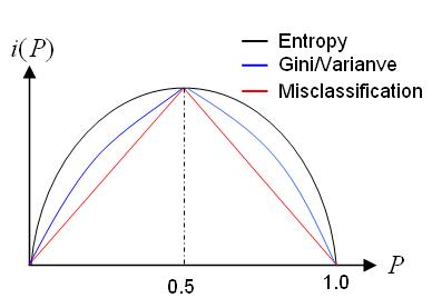
$\tau$ is most impure when$P{Y = 1 | \tau} =\frac{1}{2}$ . - The impurity function has a concave shape and can be formally defined as
$$i(\tau)=\phi(P(Y=1\mid \tau))$$ where the function$\phi$ has the properties (i)$\phi \geq 0$ and (ii) for any$p \in (0, 1)$ ,$\phi(p) = \phi(1 - p)$ and$\phi(0) = \phi(1) < \phi(p)$ .
C4.5 uses entropy for its impurity function,
whereas CART uses a generalization of the binomial variance called the Gini index.
If the training set
where
$$
Ent(D)=\sum_{y \in Y} P(y|D)\log(\frac{1}{P(y | D)}),
$$
where
The information gain ratio of features
$$
g_{R}(D,A)=\frac{G(D,A)}{Ent(D)}.
$$
And another option of impurity is Gini index of probability
| Algorithm | Splitting Criteria | Loss Function |
|---|---|---|
| ID3 | Information Gain | |
| C4.5 | Normalized information gain ratio | |
| CART | Gini Index |
If you have a constant approximation
Suppose that you have
$$L(\hat f) = (\log P(Y=Y_{observed} | X, Y_{observed}=1)) P(Y_{observed} = 1) \
- (\log P(Y=Y_{observed} | X, Y_{observed}=0)) P(Y_{observed} = 0)$$
Substituting in some variables gives $$L(\hat f) = \frac{p}{n} \log f
- \frac{n - p}{n} \log (1 - f).$$
And
A similar derivation shows that Gini impurity corresponds to a Brier score loss function. The Brier score for a candidate model
Like log-likelihood, the predictions that f^ should make to minimize the Brier score are simply
Now let’s take the expected Brier score and break up by
- \hat f(X)^2 P(Y_{observed} = 0)$$
Plugging in some values:
$$B(\hat f) = (1 - f)^2 f + f^2(1 - f) = f(1-f)$$ which is exactly (proportional to) the Gini impurity in the 2-class setting. (A similar result holds for multiclass learning as well.)
| --- | --- |
|---|---|
| QUEST | ? |
| Oblivious Decision Trees | ? |
| Online Adaptive Decision Trees | ? |
| Lazy Tree | ? |
| Option Tree | ? |
| Oblique Decision Trees | ? |
| MARS | ? |
- Building Classification Models: id3-c45
- Data Mining Tools See5 and C5.0
- A useful view of decision trees
- https://www.wikiwand.com/en/Decision_tree_learning
- https://www.wikiwand.com/en/Decision_tree
- https://www.wikiwand.com/en/Recursive_partitioning
- TimeSleuth is an open source software tool for generating temporal rules from sequential data
In this paper, we consider that the instances take the form
In a compact way, the general linear test can be rewriiten as

- https://computing.llnl.gov/projects/sapphire/dtrees/oc1.html
- Decision Forests with Oblique Decision Trees
- Global Induction of Oblique Decision Trees: An Evolutionary Approach
- On Oblique Random Forests
It is natural to generalized to nonlinear test, which can be seen as feature engineering of the input data.
- Classification and Regression Tree Methods(In Encyclopedia of Statistics in Quality and Reliability)
- Classification And Regression Trees for Machine Learning
- Classification and regression trees
- http://homepages.uc.edu/~lis6/Teaching/ML19Spring/Lab/lab8_tree.html
- CLASSIFICATION AND REGRESSION TREES AND FORESTS FOR INCOMPLETE DATA FROM SAMPLE SURVEYS
- Classification and Regression Tree Approach for Prediction of Potential Hazards of Urban Airborne Bacteria during Asian Dust Events
https://publichealth.yale.edu/c2s2/8_209304_5_v1.pdf
- https://github.com/doubleplusplus/incremental_decision_tree-CART-Random_Forest_python
- https://people.cs.umass.edu/~utgoff/papers/mlj-id5r.pdf
- https://people.cs.umass.edu/~lrn/iti/index.html
- A Streaming Parallel Decision Tree Algorithm

- Very Fast Decision Tree (VFDT) classifier
- Mining High-Speed Data Streams
- http://huawei-noah.github.io/streamDM/docs/HDT.html
- http://www.cs.washington.edu/dm/vfml/vfdt.html
- VFDT Algorithm for Decision Tree Generation
- https://www.cs.upc.edu/~gavalda/DataStreamSeminar/files/Lecture7.pdf
- Runtime Optimizations for Tree-based Machine Learning Models
- Optimized very fast decision tree with balanced classification accuracy and compact tree size
- Distributed Decision Trees with Heterogeneous Parallelism
Unlike the classical decision tree approach, this method builds a predictive model with high degree of connectivity by merging statistically indistinguishable nodes at each iteration. The key advantage of decision stream is an efficient usage of every node, taking into account all fruitful feature splits. With the same quantity of nodes, it provides higher depth than decision tree, splitting and merging the data multiple times with different features. The predictive model is growing till no improvements are achievable, considering different data recombinations, and resulting in deep directed acyclic graph, where decision branches are loosely split and merged like natural streams of a waterfall. Decision stream supports generation of extremely deep graph that can consist of hundreds of levels.
- Fast Ranking with Additive Ensembles of Oblivious and Non-Oblivious Regression Trees
- https://www.ijcai.org/Proceedings/95-2/Papers/008.pdf
- http://www.aaai.org/Papers/Workshops/1994/WS-94-01/WS94-01-020.pdf
- Decision Graphs : An Extension of Decision Trees
- https://www.projectrhea.org/rhea/index.php/ECE662:Glossary_Old_Kiwi
| Properties of Decision Tree |
|---|
| Classification and Regression Decision Trees Explained |
| linearly separable data points. |
| Limitations of Trees |
| Tree structure is prone to instability even with minor data perturbations. |
| To leverage the richness of a data set of massive size, we need to broaden the classic statistical view of “one parsimonious model" for a given data set. |
| Due to the adaptive nature of the tree construction, theoretical inference based on a tree is usually not feasible. Generating more trees may provide an empirical solution to statistical inference. |
YOSHUA BENGIO, OLIVIER DELALLEAU, AND CLARENCE SIMARD demonstrates some theoretical limitations of decision trees. And they can be seriously hurt by the curse of dimensionality in a sense that is a bit different from other nonparametric statistical methods, but most importantly, that they cannot generalize to variations not seen in the training set. This is because a decision tree creates a partition of the input space and needs at least one example in each of the regions associated with a leaf to make a sensible prediction in that region. A better understanding of the fundamental reasons for this limitation suggests that one should use forests or even deeper architectures instead of trees, which provide a form of distributed representation and can generalize to variations not encountered in the training data.
Random forests (Breiman, 2001) is a substantial modification of bagging that builds a large collection of de-correlated trees, and then averages them.
On many problems the performance of random forests is very similar to boosting, and they are simpler to train and tune.
- For
$t=1, 2, \dots, T$ :- Draw a bootstrap sample
$Z^{\ast}$ of size$N$ from the training data. - Grow a random-forest tree
$T_t$ to the bootstrapped data, by recursively repeating the following steps for each terminal node of the tree, until the minimum node size$n_{min}$ is reached.- Select
$m$ variables at random from the$p$ variables. - Pick the best variable/split-point among the
$m$ . - Split the node into two daughter nodes.
- Select
- Draw a bootstrap sample
- Vote for classification and average for regression.

Because of so many trees in a forest, it is impractical to present a forest or interpret a forest. Zhang and Wang (2009): a tree is removed if its removal from the forest has the minimal impact on the overall prediction accuracy
- Calculate the prediction accuracy of forest
$F$ , denoted by$p_F$ . For every tree, denoted by$T$ , in forest$F$ , calculate the prediction accuracy of forest$F_{−T}$ that excludes$T$ , denoted by$p_{F_{−T}}$ . - Let
$\Delta_{−T}$ be the difference in prediction accuracy between$F$ and$F_{−T} :\Delta_{−T} = p_F ??? p_{F_{−T}}$ . - The tree
$T^p$ with the smallest$\Delta_{−T}$ is the least important one and hence subject to removal:$T^p = \arg\min_{T\in F}( \Delta_{−T})$ .
Optimal Size Subforest


| properties of random forest |
|---|
| Robustness to Outliers |
| Scale Tolerance |
| Ability to Handle Missing Data |
| Ability to Select Features |
| Ability to Rank Features |
- randomForestExplainer
- https://modeloriented.github.io/randomForestExplainer/
- Awesome Random Forest
- Interpreting random forests
- Random Forests by Leo Breiman and Adele Cutler
- https://dimensionless.in/author/raghav/
- https://koalaverse.github.io/machine-learning-in-R/random-forest.html
- https://www.wikiwand.com/en/Random_forest
- https://sktbrain.github.io/awesome-recruit-en.v2/
- Introduction to Random forest by Raghav Aggiwal
- Jump Start your Modeling with Random Forests by Evan Elg
- Complete Analysis of a Random Forest Model
- Analysis of a Random Forests Model
- Narrowing the Gap: Random Forests In Theory and In Practice
- Random Forest:??? A Classification and Regression Tool for Compound Classification and QSAR Modeling

Whereas polynomial functions impose a global non-linear relationship, step functions break the range of x into bins, and fit a different constant for each bin. This amounts to converting a continuous variable into an ordered categorical variable such that our linear regression function is converted to Equation 1???
where
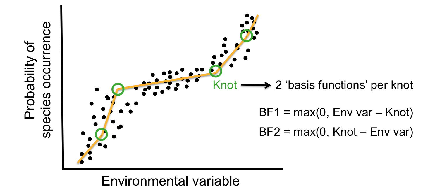
The MARS algorithm builds a model in two steps. First, it creates a collection of so-called basis functions (BF). In this procedure, the range of predictor values is partitioned in several groups. For each group, a separate linear regression is modeled, each with its own slope. The connections between the separate regression lines are called knots. The MARS algorithm automatically searches for the best spots to place the knots. Each knot has a pair of basis functions. These basis functions describe the relationship between the environmental variable and the response. The first basis function is ‘max(0, env var - knot), which means that it takes the maximum value out of two options: 0 or the result of the equation ‘environmental variable value ??? value of the knot???. The second basis function has the opposite form: max(0, knot - env var).
To highlight the progression from recursive partition regression to MARS we start by giving the partition regression model,
The usual MARS model is the same as that given in (2) except that the basis functions are different. Instead the
- http://uc-r.github.io/mars
- OVERVIEW OF SDM METHODS IN BCCVL
- https://projecteuclid.org/download/pdf_1/euclid.aos/1176347963
- Using multivariate adaptive regression splines to predict the distributions of New Zealand’s freshwater diadromous fish
- http://www.stat.ucla.edu/~cocteau/stat204/readings/mars.pdf
- Multivariate Adaptive Regression Splines (MARS)
- https://en.wikipedia.org/wiki/Multivariate_adaptive_regression_splines
- https://github.com/cesar-rojas/mars
- Earth: Multivariate Adaptive Regression Splines (MARS)
- A Python implementation of Jerome Friedman's Multivariate Adaptive Regression Splines
- https://bradleyboehmke.github.io/HOML/mars.html
- http://www.cs.rtu.lv/jekabsons/Files/ARESLab.pdf
- https://asbates.rbind.io/2019/03/02/multivariate-adaptive-regression-splines/
A Bayesian approach to multivariate adaptive regression spline (MARS) fitting (Friedman, 1991) is proposed. This takes the form of a probability distribution over the space of possible MARS models which is explored using reversible jump Markov chain Monte Carlo methods (Green, 1995). The generated sample of MARS models produced is shown to have good predictive power when averaged and allows easy interpretation of the relative importance of predictors to the overall fit.
The BMARS basis function can be written as
$$B(\vec{x}) = \beta_{0} + \sum_{k=1}^{\mathrm{K}} \beta_{k} \prod_{l=0}^{\mathrm{I}}{\left(x_{l} - t_{k, l}\right)}{+}^{o{k, l}}\tag{1}$$
where
- Bayesian MARS
- An Implementation of Bayesian Adaptive Regression Splines (BARS) in C with S and R Wrappers
- Classification with Bayesian MARS
- http://www.drryanmc.com/presentations/BMARS.pdf
- Bayesian methods for nonlinear classification and regression. (2002). Denison, Holmes, Mallick and Smith: Wiley.
- Gradient Enhanced Bayesian MARS for Regression and Uncertainty Quantification
There are many competing techniques for solving the problem, and each technique is characterized by choices and meta-parameters: when this flexibility is taken into account, one easily ends up with a very large number of possible models for a given task.
- Computer Science 598A: Boosting: Foundations & Algorithms
- 4th Workshop on Ensemble Methods
- Zhou Zhihua's publication on ensemble methods
- Online Ensemble Learning: An Empirical Study
- Ensemble Learning literature review
- KAGGLE ENSEMBLING GUIDE
- Ensemble Machine Learning: Methods and Applications
- MAJORITY VOTE CLASSIFIERS: THEORY AND APPLICATION
- Neural Random Forests
- Generalized Random Forests
- Selective Ensemble of Decision Trees
- An Empirical Comparison of Voting Classification Algorithms: Bagging, Boosting, and Variants
- DIFFERENT TYPES OF ENSEMBLE METHODS
| Bagging | Boosting | Stacking |
|---|---|---|
 |
 |
 |
- ML-Ensemble: High performance ensemble learning in Python
- https://github.com/flennerhag/mlens
- https://mlbox.readthedocs.io/en/latest/
- Ensemble Systems & Learn++ by Robi Polikar
- Applications of Supervised and Unsupervised Ensemble Methods
- Boosting-Based Face Detection and Adaptation (Synthesis Lectures on Computer Vision #2)
- Feature Selection and Ensemble Methods for Bioinformatics: Algorithmic Classification and Implementations
- Outlier Ensembles: An Introduction
Bagging, short for 'bootstrap aggregating', is a simple but highly effective ensemble method that creates diverse models on different random bootstrap samples of the original data set. Random forest is the application of bagging to decision tree algorithms.
The basic motivation of parallel ensemble methods is to exploit the independence between the base learners, since the error can be reduced dramatically by combining independent base learners. Bagging adopts the most popular strategies for aggregating the outputs of the base learners, that is, voting for classification and averaging for regression.
- Draw
bootstrap samples$B_1, B_2, \dots, B_n$ independently from the original training data set for base learners; - Train the $i$th base learner
$F_i$ at the${B}_{i}$ ; - Vote for classification and average for regression.

It is a sample-based ensemble method.
- http://www.machine-learning.martinsewell.com/ensembles/bagging/
- https://www.cnblogs.com/earendil/p/8872001.html
- https://www.wikiwand.com/en/Bootstrap_aggregating
- Bagging Regularizes
- Bootstrap Inspired Techniques in Computational Intelligence
- ranger: A Fast Implementation of Random Forests for High Dimensional Data in C++ and R
- http://rob.schapire.net/papers
- https://cseweb.ucsd.edu/~yfreund/papers
- http://www.boosting.org/
- FastForest: Learning Gradient-Boosted Regression Trees for Classification, Regression and Ranking
- Additive Models, Boosting, and Inference for Generalized Divergences
- Weak Learning, Boosting, and the AdaBoost algorithm
- http://jboost.sourceforge.net/
- The Boosting Margin, or Why Boosting Doesn’t Overfit
- Boosting Resources by Liangliang Cao
The term boosting refers to a family of algorithms that are able to convert weak learners to strong learners.
It is kind of similar to the "trial and error" scheme: if we know that the learners perform worse at some given data set

- https://mlcourse.ai/articles/topic10-boosting/
- Reweighting with Boosted Decision Trees
- https://betterexplained.com/articles/adept-method/
- BOOSTING ALGORITHMS: REGULARIZATION, PREDICTION AND MODEL FITTING
- What is the difference between Bagging and Boosting?
- Boosting and Ensemble Learning
- Boosting at Wikipedia
- Tree, Forest and Ensemble
- An Empirical Comparison of Voting Classification Algorithms: Bagging, Boosting, and Variants
- Online Parallel Boosting
| Methods | Overfit-underfitting | Training Type |
|---|---|---|
| Bagging | avoid over-fitting | parallel |
| Boosting | avoid under-fitting | sequential |
AdaBoost is a boosting methods for supervised classification algorithms, so that the labeled data set is given in the form $D={ (x_i, \mathrm{y}i)}{i=1}^{N}$.
AdaBoost is to change the distribution of training data and learn from the shuffled data.
It is an iterative trial-and-error in some sense.
Discrete AdaBoost
- Input $D={ (x_i, \mathrm{y}i)}{i=1}^{N}$ where
$x\in \mathcal X$ and$\mathrm{y}\in {+1, -1}$ . - Initialize the observation weights
${w}_i=\frac{1}{N}, i=1, 2, \dots, N$ . - For
$t = 1, 2, \dots, T$ :- Fit a classifier
$G_t(x)$ to the training data using weights$w_i$ . - Compute $$err_{t}=\frac{\sum_{i=1}^{N}w_i \mathbb{I}(G_t(x_i) \not= \mathrm{y}i)}{\sum{i=1}^{N} w_i}.$$
- Compute
$\alpha_t = \log(\frac{1-err_t}{err_t})$ . - Set $w_i\leftarrow w_i\exp[\alpha_t\mathbb{I}(G_t(x_i) \not= \mathrm{y}i)], i=1,2,\dots, N$ and renormalize so that $\sum{i}w_i=1$.
- Fit a classifier
- Output
$G(x)=sign[\sum_{t=1}^{T}\alpha_{t}G_t(x)]$ .
The indicator function
Note that the weight updating


- AdaBoost at Wikipedia
- BrownBoost at Wikipedia
- CoBoosting at Wikipedia
- CSDN blog: Adaboost 算法的原理与推导
- On the Convergence Properties of Optimal AdaBoost
- Some Open Problems in Optimal AdaBoost and Decision Stumps
- Parallelizing AdaBoost by weights dynamics

For a two-class problem, an additive logistic model has the form
where
Consider the exponential criterion
The Discrete AdaBoost algorithm (population version) builds an additive logistic regression model via Newton-like updates for minimizing
$\mathbb{E}[\exp(-yF(x))]$ .
so that
$$
\frac{\partial \mathbb{E}[\exp(-yF(x))]}{\partial F(x)} = - \exp(-F(x))P(y=+1\mid x) + \exp(F(x))P(y=-1\mid x)\tag{1}
$$
where and
So that
$$\operatorname{sign}(H(x))=\operatorname{sign}(\frac{1}{2}\log\frac{P(y=1\mid x)}{P(y=-1\mid x)})
\=\begin{cases}1,&\text{if
- Input $D={ (x_i, \mathrm{y}i)}{i=1}^{N}$ where
$x\in \mathcal X$ and$\mathrm{y}\in {+1, -1}$ . - Initialize the observation weights
${w}_i=\frac{1}{N}, i=1, 2, \dots, N$ . - For
$t = 1, 2, \dots, T$ :- Fit a classifier
$G_t(x)$ to the training data using weights$w_i$ . - Compute $$err_{t}=\frac{\sum_{i=1}^{N}w_i \mathbb{I}(G_t(x_i) \not= \mathrm{y}i)}{\sum{i=1}^{N} w_i}.$$
- Compute
$\alpha_t = \log(\frac{1-err_t}{err_t})$ . - Set $w_i\leftarrow w_i\exp[-\alpha_t G_t(x_i)\mathrm{y}i)], i=1,2,\dots, N$ and renormalize so that $\sum{i}w_i=1$.
- Fit a classifier
- Output
$G(x)=sign[\sum_{t=1}^{T}\alpha_{t}G_t(x)]$ .
In AdaBoost, the error is binary- it is 0 if the classification is right otherwise it is 1. It is not precise for some setting. The output of decision trees is a class probability estimate
Real AdaBoost
- Input $D={ (x_i, \mathrm{y}i)}{i=1}^{N}$ where
$x\in \mathcal X$ and$y\in {+1, -1}$ . - Initialize the observation weights
${w}_i=\frac{1}{N}, i=1, 2, \dots, N$ ; - For
$m = 1, 2, \dots, M$ :- Fit a classifier
$G_m(x)$ to obtain a class probability estimate$p_m(x)=\hat{P}_{w}(y=1\mid x)\in [0, 1]$ , using weights$w_i$ . - Compute
$f_m(x)\leftarrow \frac{1}{2}\log{p_m(x)/(1-p_m(x))}\in\mathbb{R}$ . - Set
$w_i\leftarrow w_i\exp[-y_if_m(x_i)], i=1,2,\dots, N$ and renormalize so that$\sum_{i=1}w_i =1$ .
- Fit a classifier
- Output
$G(x)=sign[\sum_{t=1}^{M}\alpha_{t}G_m(x)]$ .
The Real AdaBoost algorithm fits an additive logistic regression model by stagewise and approximate optimization of
$\mathbb{E}[\exp(-yF(x))]$ .
- Input $D={ (x_i, \mathrm{y}i)}{i=1}^{N}$ where
$x\in \mathcal X$ and$y\in {+1, -1}$ . - Initialize the observation weights
${w}_i=\frac{1}{N}, i=1, 2, \dots, N, F(x)=0$ ; - For
$m = 1, 2, \dots, M$ :- Fit a classifier
$f_m(x)$ by weighted least-squares of$\mathrm{y}_i$ to$x_i$ with weights$w_i$ . - Update
$F(x)\leftarrow F(x)+f_m (x)$ . - UPdate
$w_i \leftarrow w_i \exp(-\mathrm{y}_i f_m (x_i))$ and renormalize.
- Fit a classifier
- Output the classifier
$sign[F(x)]=sign[\sum_{t=1}^{M}\alpha_{t}f_m(x)]$ .
Given a training data set ${{\mathrm{X}i, y_i}}{i=1}^{N}$, where $\mathrm{X}i\in\mathbb{R}^p$ is the feature and $y_i\in{1, 2, \dots, K}$ is the desired categorical label. The classifier $F$ learned from data is a function $$ F:\mathbb{R}^P\to y \ \quad X_i \mapsto y_i. $$ And the function $F$ is usually in the additive model $F(x)=\sum{m=1}^{M}h(x\mid {\theta}_m)$.
LogitBoost (two classes)
- Input $D={ (x_i, \mathrm{y}i)}{i=1}^{N}$ where
$x\in \mathcal X$ and$y\in {+1, -1}$ . - Initialize the observation weights
${w}_i=\frac{1}{N}, i=1, 2, \dots, N, F(x)=0, p(x_i)=\frac{1}{2}$ ; - For
$m = 1, 2, \dots, M$ :- Compute the working response and weights:
$$z_i = \frac{y_i^{\ast}-p_i}{p_i(1-p_i)},\ w_i = p_i(1-p_i). $$ - Fit a classifier
$f_m(x)$ byweighted least-squaresof$\mathrm{y}_i$ to$x_i$ with weights$w_i$ . - Update
$F(x)\leftarrow F(x)+\frac{1}{2}f_m (x)$ . - UPdate
$w_i \leftarrow w_i \exp(-\mathrm{y}_i f_m (x_i))$ and renormalize.
- Compute the working response and weights:
- Output the classifier
$sign[F(x)]=sign[\sum_{t=1}^{M}\alpha_{t}f_m(x)]$ .
Here

where

- LogitBoost used first and second derivatives to construct the trees;
- LogitBoost was believed to have numerical instability problems.
- Fundamental Techniques in Big Data Data Streams, Trees, Learning, and Search by Li Ping
- LogitBoost python package
- ABC-LogitBoost for Multi-Class Classification
- LogitBoost学习
- 几种Boost算法的比较
- Robust LogitBoost and Adaptive Base Class (ABC) LogitBoost
Breiman proposes a boosting algorithm called arc-x4 to investigate whether the success of AdaBoost roots in its technical details or in the resampling scheme it uses.
The difference between AdaBoost and arc-x4 is twofold.
First, the weight for object
arc represents adaptively resample and combine.

- Combining Pattern Classifiers: Methods and Algorithms
- BIAS, VARIANCE , AND ARCING CLASSIFIERS
- Online Ensemble Learning: An Empirical Study
- Arcing Classifiers
| Properties of AdaBoost |
|---|
| AdaBoost is inherently sequential. |
| The training classification error has to go down exponentially fast if the weighted errors of the component classifiers are strictly better than chance. |
| A crucial property of AdaBoost is that it almost never overfits the data no matter how many iterations it is run. |
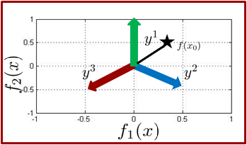
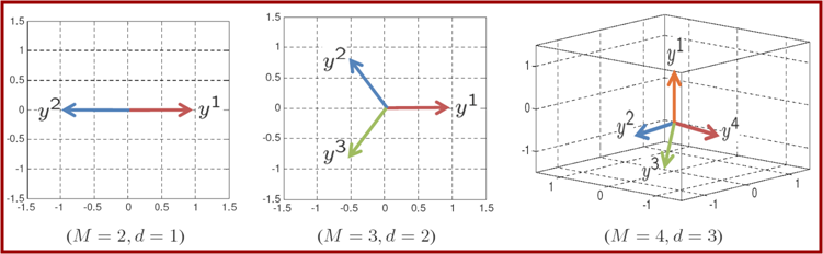
In binary classification we learn a function
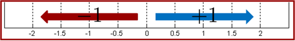
Using this observation, for multiclass boosting, e.g. 3 classes, we need to push examples in three different directions.
- Initialize the observation weights
${w}_i=\frac{1}{N}, i=1, 2, \dots, N$ . - For
$t = 1, 2, \dots, T$ :- Fit a classifier
$G_t(x)$ to the training data using weights$w_i$ . - Compute $$err_{t}=\frac{\sum_{i=1}^{N}w_i \mathbb{I}(G_t(x_i) \not= \mathrm{y}i)}{\sum{i=1}^{N} w_i}.$$
- Compute
$\alpha_t = \log(\frac{1-err_t}{err_t})+\log(K-1)$ . - Set $w_i\leftarrow w_i\exp[\alpha_t\mathbb{I}(G_t(x_i) \not= \mathrm{y}i)], i=1,2,\dots, N$ and renormalize so that $\sum{i}w_i=1$.
- Fit a classifier
- Output
$G(x)=\arg\max_{k}[\sum_{t=1}^{T}\alpha_{t}\mathbb{I}_{G_t(x)=k}]$ .


- Multiclass Boosting: MCBoost
- Multiclass Boosting: Theory and Algorithms
- multiclass boosting: theory and algorithms
- Boosting Algorithms for Simultaneous Feature Extraction and Selection
- A theory of multiclass boosting
- https://www.lri.fr/~kegl/research/publications.html
- The return of AdaBoost.MH: multi-class Hamming trees
- https://github.com/tizfa/sparkboost
- LDA-AdaBoost.MH: Accelerated AdaBoost.MH based on latent Dirichlet allocation for text categorization
- MultiBoost: A Multi-purpose Boosting Package
- http://www.multiboost.org/
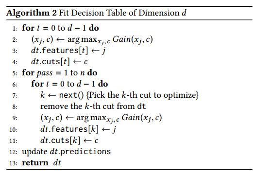
bonsai BDT (BBDT):
-
$\fbox{discretizes}$ input variables before training which ensures a fast and robust implementation - converts decision trees to n-dimentional table to store
- prediction operation takes one reading from this table
The first step of preprocessing data limits where the splits of the data can be made and, in effect, permits the grower of the tree to
control and shape its growth; thus, we are calling this a bonsai BDT (BBDT).
The discretization works by enforcing that the smallest keep interval that can be created when training the BBDT is:
Discretization means that the data can be thought of as being binned, even though many of the possible bins may not form leaves in the BBDT; thus, there are a finite number, $n^{max}{keep}$, of possible keep regions that can be defined. If the $n^{max}{keep}$ BBDT response values can be stored in memory, then the extremely large number of if/else statements that make up a BDT can be converted into a one-dimensional array of response values. One-dimensional array look-up speeds are extremely fast; they take, in essense, zero time. If there is not enough memory available to store all of the response values, there are a number of simple alternatives that can be used. For example, if the cut value is known then just the list of indices for keep regions could be stored.
- Efficient, reliable and fast high-level triggering using a bonsai boosted decision tree
- bonzaiboost documentation
- Boosting bonsai trees for efficient features combination : Application to speaker role identification
- Bonsai Trees in Your Head: How the Pavlovian System Sculpts Goal-Directed Choices by Pruning Decision Trees
- HEM meets machine learning
- BDT: Gradient Boosted Decision Tables for High Accuracy and Scoring Efficiency
- Gradient Boosted Feature Selection
- Gradient Regularized Budgeted Boosting
- Open machine learning course. Theme 10. Gradient boosting
- GBM in Machine Learning in R
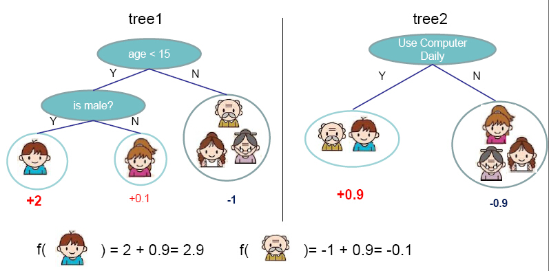
One of the frequently asked questions is What's the basic idea behind gradient boosting? and the answer from [https://explained.ai/gradient-boosting/faq.html] is the best one I know:
Instead of creating a single powerful model, boosting combines multiple simple models into a single composite model. The idea is that, as we introduce more and more simple models, the overall model becomes stronger and stronger. In boosting terminology, the simple models are called weak models or weak learners. To improve its predictions, gradient boosting looks at the difference between its current approximation,$\hat{y}$ , and the known correct target vector
${y}$ , which is called the residual,$y-\hat{y}$ . It then trains a weak model that maps feature vector${x}$ to that residual vector. Adding a residual predicted by a weak model to an existing model's approximation nudges the model towards the correct target. Adding lots of these nudges, improves the overall models approximation.
| Gradient Boosting |
|---|
 |
It is the first solution to the question that if weak learner is equivalent to strong learner.
We may consider the generalized additive model, i.e.,
$$ \hat{y}i = \sum{k=1}^{K} f_k(x_i) $$
where
$$ obj = \underbrace{\sum_{i=1}^{n} L(y_i,\hat{y}i)}{\text{error term} } + \underbrace{\sum_{k=1}^{K} \Omega(f_k)}_{regularazation} $$
where
The additive training is to train the regression tree sequentially. The objective function of the $t$th regression tree is defined as
$$ obj^{(t)} = \sum_{i=1}^{n} L(y_i,\hat{y}^{(t)}i) + \sum{k=1}^{t} \Omega(f_k) \ = \sum_{i=1}^{n} L(y_i,\hat{y}^{(t-1)}_i + f_t(x_i)) + \Omega(f_t) + C $$
where
Particularly, we take
$$ obj^{(t)} = \sum_{i=1}^{n} [y_i - (\hat{y}^{(t-1)}i + f_t(x_i))]^2 + \Omega(f_t) + C \ = \sum{i=1}^{n} [-2(y_i - \hat{y}^{(t-1)}_i) f_t(x_i) + f_t^2(x_i) ] + \Omega(f_t) + C^{\prime} $$
where $C^{\prime}=\sum_{i=1}^{n} (y_i - \hat{y}^{(t-1)}i)^2 + \sum{k=1}^{t-1} \Omega(f_k)$.
If there is no regular term
Boosting for Regression Tree
- Input training data set
${(x_i, \mathrm{y}_i)\mid i=1, \cdots, n}, x_i\in\mathcal x\subset\mathbb{R}^n, y_i\in\mathcal Y\subset\mathbb R$ . - Initialize
$f_0(x)=0$ . - For
$t = 1, 2, \dots, T$ :- For
$i = 1, 2,\dots , n$ compute the residuals$$r_{i,t}=y_i-f_{t-1}(x_i)=y_i - \hat{y}_i^{t-1}.$$ - Fit a regression tree to the targets
$r_{i,t}$ giving terminal regions$$R_{j,m}, j = 1, 2,\dots , J_m. $$ - For
$j = 1, 2,\dots , J_m$ compute $$\fbox{$\gamma_{j,t}=\arg\min_{\gamma}\sum_{x_i\in R_{j,m}}{L(\mathrm{d}i, f{t-1}(x_i)+\gamma)}$}. $ $ - Update $f_t = f_{t-1}+ \nu{\sum}{j=1}^{J_m}{\gamma}{j, t} \mathbb{I}(x\in R_{j, m}),\nu\in(0, 1)$.
- For
- Output
$f_T(x)$ .
For general loss function, it is more common that $(y_i - \hat{y}^{(t-1)}i) \not=-\frac{1}{2} {[\frac{\partial L(\mathrm{y}i, f(x_i))}{\partial f(x_i)}]}{f=f{t-1}}$.
Gradient Boosting for Regression Tree
- Input training data set
${(x_i, \mathrm{y}_i)\mid i=1, \cdots, n}, x_i\in\mathcal x\subset\mathbb{R}^n, y_i\in\mathcal Y\subset\mathbb R$ . - Initialize
$f_0(x)=\arg\min_{\gamma} L(\mathrm{y}_i,\gamma)$ . - For
$t = 1, 2, \dots, T$ :- For
$i = 1, 2,\dots , n$ compute $$r_{i,t}=-{[\frac{\partial L(\mathrm{y}i, f(x_i))}{\partial f(x_i)}]}{f=f_{t-1}}.$$ - Fit a regression tree to the targets
$r_{i,t}$ giving terminal regions$$R_{j,m}, j = 1, 2,\dots , J_m. $$ - For
$j = 1, 2,\dots , J_m$ compute $$\gamma_{j,t}=\arg\min_{\gamma}\sum_{x_i\in R_{j,m}}{L(\mathrm{d}i, f{t-1}(x_i)+\gamma)}. $$ - Update $f_t = f_{t-1}+ \nu{\sum}{j=1}^{J_m}{\gamma}{j, t} \mathbb{I}(x\in R_{j, m}),\nu\in(0, 1)$.
- For
- Output
$f_T(x)$ .
An important part of gradient boosting method is regularization by shrinkage which consists in modifying the update rule as follows: $$ f_{t} =f_{t-1}+\nu \underbrace{ \sum_{j = 1}^{J_{m}} \gamma_{j, t} \mathbb{I}(x\in R_{j, m}) }{ \text{ to fit the gradient} }, \ \approx f{t-1} + \nu \underbrace{ {\sum}{i=1}^{n} -{[\frac{\partial L(\mathrm{y}i, f(x_i))}{\partial f(x_i)}]}{f=f{t-1}} }_{ \text{fitted by a regression tree} }, \nu\in(0,1). $$
Note that the incremental tree is approximate to the negative gradient of the loss function, i.e.,
$$\fbox{ $\sum_{j=1}^{J_m} \gamma_{j, t} \mathbb{I}(x\in R_{j, m}) \approx {\sum}{i=1}^{n} -{[\frac{\partial L(\mathrm{y}i, f(x_i))}{\partial f(x_i)}]}{f=f{t-1}}$ }$$
where
Method | Hypothesis space| Update formulea | Loss function
---|---|---|---|---
Gradient Descent | parameter space
- Greedy Function Approximation: A Gradient Boosting Machine
- Gradient Boosting at Wikipedia
- Gradient Boosting Explained
- Gradient Boosting Interactive Playground
- https://www.ncbi.nlm.nih.gov/pmc/articles/PMC3885826/
- https://explained.ai/gradient-boosting/index.html
- https://explained.ai/gradient-boosting/L2-loss.html
- https://explained.ai/gradient-boosting/L1-loss.html
- https://explained.ai/gradient-boosting/descent.html
- https://explained.ai/gradient-boosting/faq.html
- GBDT算法原理 - 飞奔的猫熊的文章 - 知乎
- https://homes.cs.washington.edu/~tqchen/pdf/BoostedTree.pdf
- https://github.com/benedekrozemberczki/awesome-gradient-boosting-papers
- https://github.com/talperetz/awesome-gradient-boosting
- https://github.com/parrt/dtreeviz
| Ensemble Methods | Training Data | Decision Tree Construction | Update Formula |
|---|---|---|---|
| AdaBoost | Fit a classifier |
||
| Gradient Boost | Fit a tree |
|
Note that
A minor modification was made to gradient boosting to incorporate randomness as an integral part of the procedure. Specially, at each iteration a subsample of the training data is drawn at random (without replacement) from the full training data set. This randomly selected subsamples is then used, instead of the full sample, to fit the base learner and compute the model update for the current iteration.
Stochastic Gradient Boosting for Regression Tree
- Input training data set ${(x_i, \mathrm{y}i)\mid i=1, \cdots, n}, x_i\in\mathcal x\subset\mathbb{R}^n, y_i\in\mathcal Y\subset\mathbb R$. Amd ${{\pi(i)}}1^N$ be a random permutation of their integers ${1,\dots, n}$. Then a random sample of size $\hat n< n$ is given by ${(x{\pi(i)}, \mathrm{y}{\pi(i)})\mid i=1, \cdots, \hat n}$.
- Initialize
$f_0(x)=\arg\min_{\gamma} L(\mathrm{y}_i,\gamma)$ . - For
$t = 1, 2, \dots, T$ :- For
$i = 1, 2,\dots , \hat n$ compute $$r_{\pi(i),t}=-{[\frac{\partial L(\mathrm{y}{\pi(i),t}, f(x{\pi(i),t}))}{\partial f(x_{\pi(i),t})}]}{f=f{t-1}}.$$ - Fit a regression tree to the targets
$r_{\pi(i),t}$ giving terminal regions$$R_{j,m}, j = 1, 2,\dots , J_m. $$ - For
$j = 1, 2,\dots , J_m$ compute $$\gamma_{j,t}=\arg\min_{\gamma}\sum_{x_{\pi(i)}\in R_{j,m}}{L(\mathrm{d}i, f{t-1}(x_{\pi(i)})+\gamma)}. $$ - Update $f_t = f_{t-1}+ \nu{\sum}{j=1}^{J_m}{\gamma}{j, t} \mathbb{I}(x\in R_{j, m}),\nu\in(0, 1)$.
- For
- Output
$f_T(x)$ .
- https://statweb.stanford.edu/~jhf/ftp/stobst.pdf
- https://statweb.stanford.edu/~jhf/
- Stochastic gradient boosted distributed decision trees
In Gradient Boost, we compute and fit a regression a tree to
$$
r_{i,t}=-{ [\frac{\partial L(\mathrm{d}i, f(x_i))}{\partial f(x_i)}] }{f=f_{t-1}}.
$$
Why not the error
In general, we can expand the objective function at
$$ obj^{(t)} = \sum_{i=1}^{n} L[y_i,\hat{y}^{(t-1)}i + f_t(x_i)] + \Omega(f_t) + C \ \simeq \sum{i=1}^{n} \underbrace{ [L(y_i,\hat{y}^{(t-1)}_i) + g_i f_t(x_i) + \frac{h_i f_t^2(x_i)}{2}