For more information see the Wikipedia page.
To every outcome
$\omega$ we now assign – according to a certain rule – a function of time$\xi(\omega, t)$ , real or complex. We have thus created a family of functions, one for each$\omega$ . This family is called a stochastic process (or a random function). from the little book
For example, if
| Stochastic Process and Management |
|---|
 |
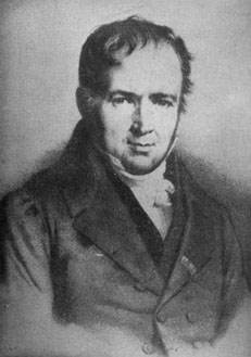
Poisson process is named after the statistician Siméon Denis Poisson.
Definition:The homogeneous Poisson point process, when considered on the positive half-line, can be defined as a counting process, a type of stochastic process, which can be denoted as
${N(t),t\geq 0}$ . A counting process represents the total number of occurrences or events that have happened up to and including time$t$ . A counting process is a Poisson counting process with rate$\lambda >0$ if it has the following three properties:
-
$N(0)=0$ ; - has independent increments, i.e.
$N(t)-N(t-\tau)$ and$N(t+\tau)-N(t)$ are independent for$0\leq\tau\leq{t}$ ; and - the number of events (or points) in any interval of length
$t$ is a Poisson random variable with parameter (or mean)$\lambda t$ .
| Siméon Denis Poisson |
|---|
 |
It is a discrete distribution with the pmf:
$$
P(X=k)=e^{-\lambda}\frac{\lambda^k}{k!}, k\in{0,1,\cdots},
$$
where
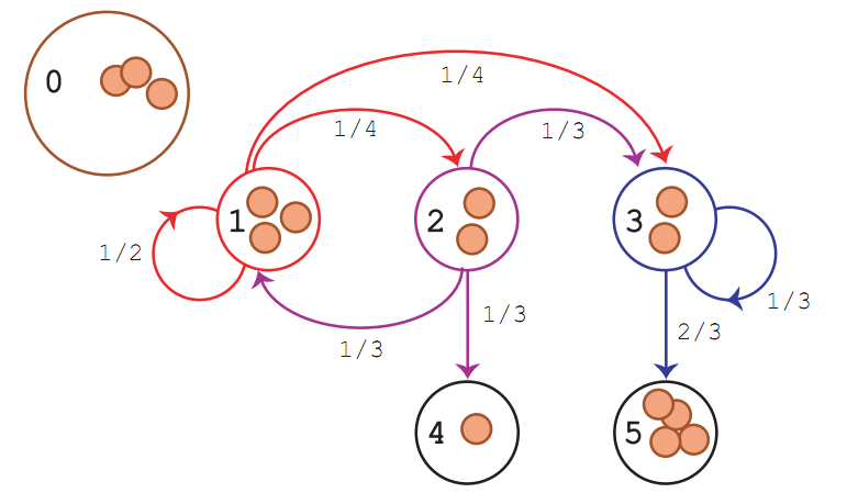
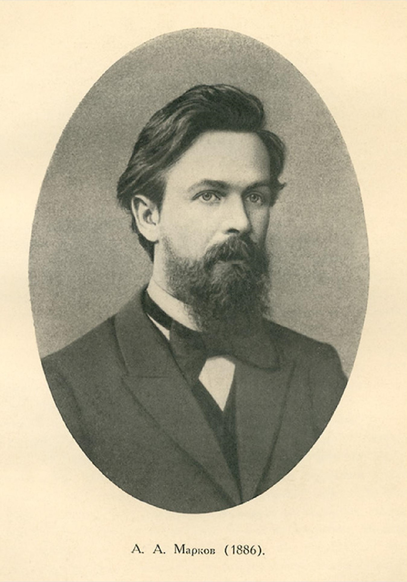
Markov chain is a simple stochastic process in honor of Andrey (Andrei) Andreyevich Marko. It is the fundamental of Markov Chain Montel Carlo(MCMC).
Definition: The process
$X$ is a Markov chain if it satisfies the Markov condition:$$P(X_{n}=x_{n}|X_{1}=x_{1},\cdots,X_{n-1}=x_{n-1})=P(X_{n}=x_{n}|X_{n-1}=x_{n-1})$$ for all$n\geq 1$ .
People introduced to Markov chains through a typical course on stochastic processes have
usually only seen examples where the state space is finite or countable. If the state space
is finite, written
and the transition probabilities can be associated with a matrix
When the state space is countably infinite, we can think of an infinite vector and matrix. And

But most Markov chains of interest in MCMC have uncountable state space, and then we cannot think of the initial distribution as a vector or the transition probability distribution as a matrix. We must think of them as an unconditional probability distribution and a conditional probability distribution.
A stochastic process is stationary if for every positive integer
An initial distribution is said to be stationary or invariant or equilibrium for some transition probability distribution if the Markov chain specified by this initial distribution and transition probability distribution is stationary. We also indicate this by saying that the transition probability distribution preserves the initial distribution.
Stationarity implies stationary transition probabilities, but not vice versa.
Let
It is the largest eigenvalue problem of the transition matrix Anderson acceleration may speed up the convergence in its iterative computational process.
A transition probability distribution is reversible with respect to an initial distribution if, for
the Markov chain
A Markov chain is reversible if its transition probability is reversible with respect to its initial distribution. Reversibility implies stationarity, but not vice versa. A reversible Markov chain has the same laws running forward or backward in time, that is, for any
| Andrey (Andrei) Andreyevich Markov,1856-1922 |
|---|
 |
| his short biography in .pdf file format |
| Hamiltonian Monte Carlo explained |
A random walk on a directed graph consists of a sequence of vertices generated from a start vertex by selecting an edge, traversing the edge to a new vertex, and repeating the process. From Foundations of Data Science
| Random Walk | Markov Chain |
|---|---|
| graph | stochastic process |
| vertex | state |
| strongly connected | persistent |
| aperiodic | aperiodic |
| strongly connected and aperiodic | ergotic |
| undirected graph | time reversible |
A random walk in the Markov chain starts at some state. At a given time step, if it is in state
A state of a Markov chain is persistent if it has the property that should the state ever
be reached, the random process will return to it with probability
A connected Markov Chain is said to be aperiodic if the greatest common divisor of the lengths of directed cycles is
The hitting time
In an undirected graph where
Thus the Metropolis-Hasting algorithm and Gibbs sampling both involve random walks on edge-weighted undirected graphs.
Definition: Let
- (a) If the current state is
${i}$ , the time until the state is changed has an exponential distribution with parameter$\lambda(i)$ . - (b) When state
${i}$ is left, a new state$j\neq i$ is chosen according to the transition probabilities of a discrete-time Markov chain.
Then
- Markov property:
$P(X(t)=j\mid X(t_1)=i_1,\dots, X(t_n)=i_n)=P(X(t)=j\mid X(t_n)=i_n)$ for any$n>1$ and$t_1<t_2<\cdots<t_n<t$ . - Time Homogeneity:
$P(X(t)=j\mid X(s)=i) = P(X(t-1)=j\mid X(0)=i)$ for$0<s<t$ .
And discrete stochastic process is matrix-based computation while the stochastic calculus is the blend of differential equation and statistical analysis.
Define
So that
Therefore, by taking first order Taylor expansion of
Let Q be the matrix of
Description of process
Let
Embedded Markov Chain
If the process is observed only at jumps, then a Markov chain is observed with transition matrix $$ P=\begin{pmatrix} \ddots & -\frac{q_{ij}}{q_{ii}} &-\frac{q_{ij}}{q_{ii} } &\cdots \ -\frac{q_{ij}}{q_{ii}} & 0 &-\frac{q_{ij}}{q_{ii}} &\cdots \ \vdots & -\frac{q_{ij}}{q_{ii}} & 0 &\cdots \ \vdots & \cdots & \cdots &\cdots \end{pmatrix} $$
known as the Embedded Markov Chain.
Forward and Backward Equations
Given Q, how do we get
- MA8109 Stochastic processes and differential equations
- Martingales and the ItÙ Integral
- Continuous time Markov processes
- Course information, a blog, discussion and resources for a course of 12 lectures on Markov Chains to second year mathematicians at Cambridge in autumn 2012.
- Markov Chains: Engel's probabilistic abacus
- Reversible Markov Chains and Random Walks on Graphs by Aldous
- Markov Chains and Mixing Times by David A. Levin, Yuval Peres, Elizabeth L. Wilmer
- Random walks and electric networks by Peter G. Doyle J. Laurie Snell
- The PageRank Citation Ranking: Bringing Order to the Web
- 能否通俗的介绍一下Hamiltonian MCMC?
Time series analysis is the statistical counterpart of stochastic process in some sense. In practice, we may observe a series of random variable but its hidden parameters are not clear before some computation. It is the independence that makes the parameter estimation of statistical models and time series analysis, which will cover more practical consideration.
A brief history of time series analysis
The theoretical developments in time series analysis started early with stochastic processes. The first actual application of autoregressive models to data can be brought back to the work of G. U Yule and J. Walker in the 1920s and 1930s.
During this time the moving average was introduced to remove periodic fluctuations in the time series, for example fluctuations due to seasonality. Herman Wold introduced ARMA (AutoRegressive Moving Average) models for stationary series, but was unable to derive a likelihood function to enable maximum likelihood (ML) estimation of the parameters.
It took until 1970 before this was accomplished. At that time, the classic book "Time Series Analysis" by G. E. P. Box and G. M. Jenkins came out, containing the full modeling procedure for individual series: specification, estimation, diagnostics and forecasting.
Nowadays, the so-called Box-Jenkins models are perhaps the most commonly used and many techniques used for forecasting and seasonal adjustment can be traced back to these models.
The first generalization was to accept multivariate ARMA models, among which especially VAR models (Vector AutoRegressive) have become popular. These techniques, however, are only applicable for stationary time series. However, especially economic time series often exhibit a rising trend suggesting non-stationarity, that is, a unit root.
Tests for unit roots developed mainly during the 1980:s. In the multivariate case, it was found that non-stationary time series could have a common unit root. These time series are called cointegrated time series and can be used in so called error-correction models within both long-term relationships and short-term dynamics are estimated.
ARCH and GARCH models Another line of development in time series, originating from Box-Jenkins models, are the non-linear generalizations, mainly ARCH (AutoRegressive Conditional Heteroscedasticity) - and GARCH- (G = Generalized) models. These models allow parameterization and prediction of non-constant variance. These models have thus proved very useful for financial time series. The invention of them and the launch of the error correction model gave C. W. J Granger and R. F. Engle the Nobel Memorial Prize in Economic Sciences in 2003.
Other non-linear models impose time-varying parameters or parameters whose values changes when the process switches between different regimes. These models have proved useful for modeling many macroeconomic time series, which are widely considered to exhibit non-linear characteristics.