Depth Camera Sonar with Normals

We are creating a Sonar model that takes into account the distance and normal angle to targets as well as frequency and beam width characteristics to calculate sonar beam reflectivity. We are testing this model in a tank environment consisting of a Sonar device, a target, and a tank, where the transmitter is offset to the left and angled to the right to add context for depth readings:

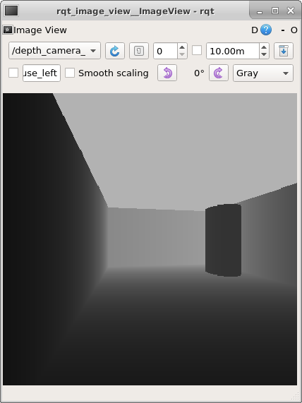
Here is this view as seen by the depth camera. Darker points are closer and lighter points are further away. The gray above is set to the cutoff distance, 7 meters. The view shown is 1.6 radians square:

We are currently hard coding a Sonar model of 16 beams along the azimuth, where each beam is calculated from a matrix of rays 3 wide by 4 high for a matrix of 48 by 4 (192 rays total) and beams are 0.1 radian wide. Here is the depth view showing this 48 by 4 matrix taken across the center strip of the depth image shown above:

Here is the view of the incidence angles, which take into account the angle of the target and the angle of the ray with respect to the angle of each sonar beam sensor:

Here is the Sonar view calculated using the 48 by 4 matrix of rays and the 48 by 4 matrix of Normals. Bars in the column furthest to the left indicate reflections for the leftmost Sonar beam. Bars in the column furthest to the right indicate reflections from the 16'th Sonar beam. There are 16 columns, one per beam. Bars at the top show closest reflections and bars at the bottom show the longest reflections. Bars values are produced by summing beam powers into 300 buckets. From left to right, reflections are from the left wall, the back wall, the target, and the right wall. Reflections are calculated about once every 10 seconds:

Although the image is drawn rectangularly, it could be drawn as a pie shape because the Sonar sensor is modeled as a point, not as a beam along the bottom.

Here is the sound pressure level chart for these 16 beams:

As noted above, calculation time takes too long. When calculating beam reflection values, computation time increases by the square of the difference between the nearest and furthest target distances. For example for targets between 0.5 and 20 meters away, each ray requires 31,467 iterations to compute reflected power. Computing all 192 rays takes 35 seconds. For targets between 0.5 and 6 meters away, each ray requires 9,440 iterations and computation takes 11 seconds.

We need to cut down the computational burden from 10 seconds to somewhere below 10 ms. If we calculate reflectivity using less iterations per beam, we would get data loss and we would need to adjust the equations for correct timing values. We may need to use look-up tables instead of iterating over frequencies. We add random noise when iterating over frequencies per beam. If we use look-up tables, we will need to apply random noise to vector data retrieved from lookup tables.

Demo

This demo may be run by typing the following:

roslaunch nps_uw_sensors_gazebo depth_camera_sonar_basic.launch

Outputs:

• The Sonar beam image is output as ROS topic sonar_beam_image of type Image.
• For diagnostics, the incidence of each ray is output as ROS topic sonar_ray_incidence_image of type Image.
• Depth values from Gazebo are output as ROS topic /depth_camera_sonar_sensor_camera/image_depth.
• Normals from Gazebo are output as ROS topic /depth_camera_sonar_sensor_camera/image_normals of type Image, but they are not viewable; each normal value is encoded in four floats.
• The sound pressure level chart is drawn in its own window. It may be enabled by uncommenting line # show_plots = True in file scripts/sonar_equations.py.